
Spatial Autocorrelation with PySAL
Last updated on 2026-10-25 | Edit this page
Overview
Questions
- What does it mean for data to be spatially autocorrelated?
- How do we tell the computer which places are neighbors?
- How do Global and Local Moran’s I measure and locate clustering?
- What choices and pitfalls affect the results?
Objectives
- Build Rook, Queen and K-nearest neighbor spatial weights with PySAL
- Compute and interpret Global Moran’s I and its p-value
- Read a Moran scatterplot
- Map statistically significant hotspots and coldspots with Local Moran’s I (LISA)
- Explain permutation tests, multiple testing and the modifiable areal unit problem
Why spatial autocorrelation?
“Everything is related to everything else, but near things are more related than distant things.” (Tobler’s first law of geography)
Most statistics assume observations are independent. Places are not: a county’s income or median age is usually similar to its neighbors’. Spatial autocorrelation measures how strong that similarity is, and PySAL (the Python Spatial Analysis Library) provides the standard tools.
| Question | PySAL method |
|---|---|
| Who counts as a neighbor? | Spatial weights (libpysal.weights) |
| Is there clustering across the whole map? | Global Moran’s I (esda.Moran) |
| Where are the hotspots and coldspots? | Local Moran’s I, LISA (esda.Moran_Local) |
| Could the pattern be chance? | Permutation tests (p_sim) |
In this episode we use 2023 American Community Survey data for Indiana counties, loaded with a Census API key (see the Census data session for how to get one).
Why it matters
Spatial autocorrelation is both a problem and a finding.
-
A problem for standard statistics. Regression and
t-tests assume that each observation adds new, independent information.
When neighbors are similar, Indiana’s 92 counties carry less independent
information than 92 random draws, so standard errors come out too small
and results look more significant than they are. Spatial regression
models (in PySAL’s
spregpackage) correct for this. - A finding in itself. Clustering says something about the process behind the data: people with similar incomes sort into similar neighborhoods, diseases spread to nearby places, and policies spill across borders. Mapping where clusters are is often the first step of a spatial study.
Spatial weights: who is a neighbor?
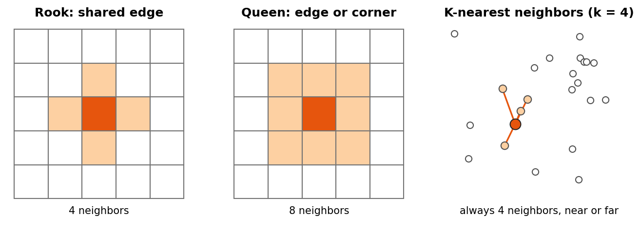
Before PySAL can compare a place with its neighbors, you must say who the neighbors are. This is the spatial weights matrix \(W\): a table with one row and one column per place, where \(w_{ij}\) is not zero when \(j\) is a neighbor of \(i\).
| Type | Neighbors are | Good for |
|---|---|---|
| Rook contiguity | Polygons that share an edge | Regular polygons and grids |
| Queen contiguity | Polygons that share an edge or a corner | Most polygon data, such as counties or tracts (the usual default) |
| K-nearest neighbors (KNN) | The k closest centers | Points, or polygons of very different sizes; every place gets exactly k neighbors |
| Distance band | Every place within a set distance | Points, when “near” has a natural distance |
Two more ideas come up constantly:
-
Row standardization
(
w.transform = "R") divides each row by the number of neighbors, so each place’s weights sum to 1. A county with eight neighbors and a county with three are then treated alike, and multiplying the weights by the data gives the spatial lag: the average value of each place’s neighbors. - Islands are places with no neighbors under a contiguity rule, such as an island county. PySAL warns about them. Drop them, or give them neighbors with a KNN or distance rule.
1. Build spatial weights
counties is a GeoDataFrame of Indiana counties with a
median_age column, projected to meters.
PYTHON
from libpysal.weights import Rook, Queen, KNN

w_rook = Rook.from_dataframe(counties, use_index=True)    # shared edge
w_queen = Queen.from_dataframe(counties, use_index=True)  # shared edge or corner
w_knn = KNN.from_dataframe(counties, k=4)                 # 4 closest centers

print(w_rook.mean_neighbors, w_queen.mean_neighbors)
w_queen.transform = "R"    # row standardize: each county's weights sum to 1
2. Global Moran’s I
PYTHON
from esda.moran import Moran

mi = Moran(counties["median_age"], w_queen, permutations=999)
print(f"I = {mi.I:.3f}, p = {mi.p_sim:.3f}")- I clearly above 0 with p below 0.05: similar values cluster together
- I near 0: no spatial pattern
- I below 0: neighbors tend to be different
Reading the Moran scatterplot
The scatterplot puts each county’s value on the x axis and its spatial lag (the average of its neighbors) on the y axis, both standardized so that 0 is the mean.
- The slope of the fitted line equals Moran’s I (with row standardized weights).
- The four quadrants are the categories that LISA uses below: top right High-High (a high value among high neighbors), bottom left Low-Low, top left Low-High (a low value among high neighbors) and bottom right High-Low.
- Points far from the line are places that do not fit the overall pattern, and are worth a closer look.
You can compute the spatial lag yourself:
Could it be chance? Permutation tests
PySAL tests significance by permutation. It shuffles the values randomly among the places, for example 999 times, recomputes I for each shuffled map, and counts how often a shuffled map is at least as extreme as the real one. The pseudo p-value is
\[ p = \frac{M + 1}{R + 1} \]
where \(M\) is the number of
shuffled maps at least as extreme as the observed one and \(R\) is the number of permutations. With 999
permutations the smallest possible p-value is 0.001. Because the
shuffles are random, p-values can change slightly from run to run;
Moran_Local accepts a seed so that results are
repeatable.
3. Local Moran’s I (LISA)
PYTHON
from esda.moran import Moran_Local
from splot.esda import lisa_cluster

lisa = Moran_Local(counties["median_age"], w_queen, permutations=999, seed=42)
lisa_cluster(lisa, counties, p=0.05)     # only significant counties are colored
Labels: High-High (hotspot), Low-Low (coldspot), High-Low and Low-High (outliers), and Not significant.
Local results need care
Local Moran’s I runs one test per place: 92 tests for Indiana counties, and hundreds or thousands for tracts. With a cutoff of p < 0.05, about 1 place in 20 would look significant even on a completely random map. To be careful:
- use a stricter cutoff, such as
p=0.01; - apply a False Discovery Rate (FDR) correction, which lowers the cutoff according to the number of tests;
- treat significant clusters as places to investigate, not as proof.
Getis-Ord Gi* (esda.G_Local) is another common hotspot
statistic. It finds clusters of high or low values but does not separate
outliers the way LISA does.
Challenge 1: Rook or Queen?
Print the Rook and Queen neighbors of the same county, for example
w_rook.neighbors[0] and w_queen.neighbors[0].
Why can Queen never have fewer neighbors than Rook?
Queen counts every county that shares an edge (like Rook) plus any that only touch at a corner. So it always includes all Rook neighbors, and sometimes a few more.
Challenge 2: A second variable
Compute Global Moran’s I for pct_asian. Is it clustered?
Then make its LISA map.
Pitfalls
- The modifiable areal unit problem (MAUP). Results change with the units. The same people aggregated to counties, tracts or ZIP codes can show different clusters, or none. State the units you used and, if you can, check another.
- Small numbers. Rates and estimates for places with small populations swing widely by chance and can create false hotspots. American Community Survey estimates for small areas also have large margins of error. Look at population sizes and margins of error before interpreting a cluster.
- Edge effects. Places on the edge of the study area, such as border counties, have fewer neighbors, so their local statistics rest on less information.
- The weights are a choice. Rook, Queen and KNN can give different answers. Try more than one; robust patterns survive the change.
- Clustering is not causation. A High-High cluster of median age says where older populations are, not why.
Challenge 3: An outlier tract
A LISA map of median household income for Marion County tracts shows one tract labeled High-Low. What does that label mean, and what could explain it? What would you check before writing about it?
High-Low means the tract’s income is well above the mean while its neighbors’ average is below the mean, and the difference is unlikely to be chance under the permutation test. It could be a new upscale development, a gentrifying area, or an affluent enclave next to lower-income neighborhoods. It could also be a statistical artifact: check the tract’s population and the estimate’s margin of error, because a small tract with a large margin of error can produce an extreme value by chance. With hundreds of tracts, also remember that about 1 in 20 can be significant at p < 0.05 by chance alone.
Math
Global Moran’s I is
\[ I = \frac{N}{W} \cdot \frac{\sum_i \sum_j w_{ij}(x_i - \bar{x})(x_j - \bar{x})}{\sum_i (x_i - \bar{x})^2} \]
where \(N\) is the number of places, \(w_{ij}\) is the weight between places \(i\) and \(j\) (non zero only for neighbors), \(W\) is the sum of all weights, and \(x\) is the variable. The top of the fraction is large when neighbors are on the same side of the mean.
- Spatial weights define who is a neighbor: Rook (edges), Queen (edges and corners), KNN (closest)
- Global Moran’s I gives one number for clustering across the whole map
- The permutation p-value tells you whether the pattern could be chance
- Local Moran’s I (LISA) locates hotspots, coldspots and outliers; always filter by p-value
- Many local tests produce false positives; use stricter cutoffs or FDR, and treat clusters as leads
- Results depend on the units (MAUP), the weights, small populations and edges of the study area
Notebooks
| Level | Notebook | What you will do |
|---|---|---|
| Beginner | 2a. What Is a Neighbor? Spatial Weights | Load Indiana counties and compare Rook, Queen and KNN neighbors |
| Intermediate | 2b. Global Moran’s I | Test whether median age is clustered and read the Moran scatterplot |
| Advanced | 2c. Local Moran’s I and Hotspots | Map significant clusters for counties, then for Marion County tracts |