
Exercise 1A: Acquiring Data and Making Your First Map in QGIS
Last updated on 2026-10-20 | Edit this page
Overview
Questions
- How do I load spatial data into QGIS?
- How can I add different types of vector data (shapefiles, CSV files, and live OSM data) to a map?
- How do I style and symbolize data to communicate clearly?
- How do I build and export a finished, publication-ready map layout?
Objectives
- Load and explore spatial datasets from multiple sources
- Install and use QGIS plugins to extend functionality
- Style layers using Single Symbol, Categorized, and Graduated options
- Build a map layout with all essential map elements
- Export a publication-ready map as an image or PDF
- QGIS can load vector data from shapefiles, GeoJSON files, geocoded CSV files, and live OpenStreetMap queries.
- Layer order matters: drag layers so that points and polygons of interest sit above basemap layers.
- Styling choices (symbol, color, size) should serve the map’s purpose, not just look decorative.
- A complete map layout includes a title, legend, scale bar, north arrow, and data source credit.
- Save your project frequently using
.qgz: losing work to an unsaved session is the most common beginner mistake.
Introduction
QGIS is a free, open-source Geographic Information System that runs on Windows, macOS, and Linux. In this episode we will go from a blank project to a finished, exported map using real spatial data.
The walkthrough below covers the core workflow: loading a shapefile, styling it, and building a map layout. The exercises that follow introduce additional data types (CSV files and live OpenStreetMap data) and give you practice combining multiple layers into a single map.
Part 1: Loading Data
Step 0: Create a Project Folder
Before opening QGIS, create a folder on your desktop called
Session_1a. All data files you download will go here,
and your QGIS project file (.qgz) will be saved here too.
Keeping data and project files together prevents broken layer links
later.
Step 1: Add a Basemap
- In the Browser Panel, expand XYZ Tiles. (If you do not see the Browser Panel, open it with View → Panels → Browser.)
- Right-click OpenStreetMap and select Add Layer to Project.
- A world map should now appear in the Map Panel.
Step 2: Download and Add a Shapefile
We will use the airports of Alaska from the QGIS sample dataset.
A shapefile is not a single file. It is a set of files with the same name, and the layer only loads correctly when all of them sit together in one folder:
| File | Purpose |
|---|---|
airports.shp |
Geometry (the point locations) |
airports.dbf |
Attribute table (the data) |
airports.prj |
Coordinate reference system |
airports.shx |
Spatial index |
airports.cpg |
Character encoding |
To make this easy, the five files are packed into one zip file:
- Download airports.zip and save it in your Session_1a folder.
- Unzip it. On Windows, right-click the file and choose
Extract All; on a Mac, double-click it. You now have a
folder called
airportsthat contains the five files.
(The original files are in the shapefiles folder of the
QGIS
Sample Data repository.)
To add the shapefile to your map:
- Go to Layer → Add Layer → Add Vector Layer.
- Under Source, click the … button,
open the
airportsfolder and selectairports.shp. - Click Add, then close the dialog.
- In the Layers Panel, drag the
airportslayer above the OpenStreetMap layer so the airport points appear on top of the basemap. - Right-click the
airportslayer and choose Zoom to Layer. The map moves to Alaska and you should see 76 points.
Why does Alaska look so big?
The OpenStreetMap basemap uses the Web Mercator projection, which stretches areas near the poles, so Alaska looks much larger than it is. The airports file itself is stored in a projection made for Alaska (NAD27 / Alaska Albers, EPSG:2964), and QGIS converts it on the fly so the points line up with the basemap. Nothing is wrong with your data.
Layer Order Matters
QGIS draws layers from bottom to top. If your data layer is underneath the basemap in the Layers Panel, it will be hidden. Always check that your data sits above any basemap layers.
Step 3: Explore the Attribute Table
The attribute table contains the data values behind every feature on the map. To open it:
- Right-click the
airportslayer in the Layers Panel. - Select Open Attribute Table.
- You should see 76 rows: one for each airport in Alaska.
Explore the columns: NAME (the airport name),
ELEV (elevation in feet), USE (how the airport
is used: Civilian/Public, Military, Joint Military/Civilian or Other),
and two ID fields. USE and ELEV are the fields
you will style the map with in the next section. Click a column header
to sort by it.
Save Often
Go to Project → Save (or Ctrl+S / Cmd+S) regularly. QGIS does not autosave. Losing progress to an unsaved session is the single most common beginner mistake.
Part 2: Styling Your Map
Step 1: Open Layer Properties
Right-click the airports layer →
Properties → navigate to the Symbology
tab.
Step 2: Choose a Symbol Style
QGIS offers three main styling modes:
| Style | Use when… | Example |
|---|---|---|
| Single Symbol | All features should look the same | All airports shown as identical blue dots |
| Categorized | Features belong to named groups | Airports colored by USE (Civilian/Public, Military,
Joint Military/Civilian, Other) |
| Graduated | Features vary along a numeric scale | Airport symbols sized by elevation (ELEV) |
For the airports layer, try Single Symbol first to get comfortable with the controls. You can adjust the marker shape, size, color, and transparency from this panel.
Then try Categorized:
- At the top of the Symbology tab, change Single Symbol to Categorized.
- Set Value to
USE. - Click Classify, then Apply. Each of the four airport uses gets its own color; double-click a symbol in the list to change it.
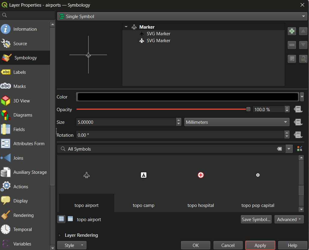
Tip: Set the Magnifier at the bottom of the Map Panel to 75% if the map feels too large for your screen.
Tip: To rename a layer (which also controls how it appears in the legend), right-click the layer → Properties → Source → Layer Name. Give it a clear, human-readable name before building your layout.
Step 3: Apply a Graduated Style (Optional: for numeric data)
Graduated symbology is useful when your data has a meaningful numeric
field. The airports layer has one, ELEV (elevation in
feet), so no extra download is needed:
- Open the airports layer’s Symbology tab and select Graduated.
- Set Value to
ELEV. - Set Method to Size (higher airports get bigger symbols), or keep Color and choose a sequential color ramp (light to dark).
- Set Classes to 5, click Classify, then Apply.
This is the same graduated approach you would use for a choropleth map of Census data or any other continuous numeric variable.
Part 3: Creating a Map Layout
The Print Layout is QGIS’s dedicated tool for building finished, export-ready maps. It is separate from the main map canvas: the main canvas is for exploration, the Print Layout is for publication.
Step 1: Open a New Layout
- Go to Project → New Print Layout (or click the New Print Layout icon in the toolbar).
- Give the layout a name and click OK.
- A new window will open with a blank white canvas representing your page.
Step 2: Add the Map Frame
- In the toolbar on the left side of the Layout window, click Add Item → Add Map.
- Draw a rectangle on the canvas by clicking and dragging. The current map view from your main canvas will appear inside the rectangle.
- Use the Item Properties panel on the right to lock the scale or adjust the extent if needed.
Step 3: Add All Required Map Elements
A complete, publication-ready map must include the following elements. Use the Add Item menu in the toolbar to insert each one:
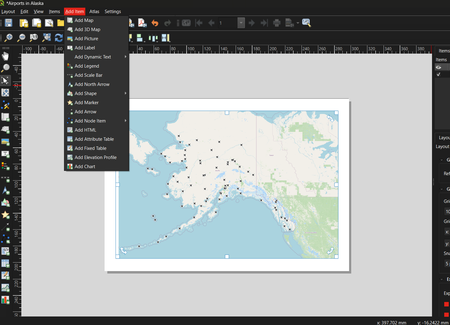
| Element | How to add | Notes |
|---|---|---|
| Title | Add Item → Add Label | Draw a text box at the top of the canvas; enter a descriptive title |
| Legend | Add Item → Add Legend | QGIS auto-populates from layer names: this is why renaming layers matters |
| Scale Bar | Add Item → Add Scale Bar | Choose units appropriate for your map extent |
| North Arrow | Add Item → Add North Arrow | Only strictly necessary if north is not obviously up |
| Data credit / metadata | Add Item → Add Label | Add at the bottom: your name, data sources, and date |
Step 4: Export the Layout
Once you are satisfied with the layout:
- Go to Layout → Export as Image (for PNG/JPEG) or Layout → Export as PDF.
- Accept the default settings and click OK.
- Return to the main QGIS window and save your project:
Project → Save (
.qgz).
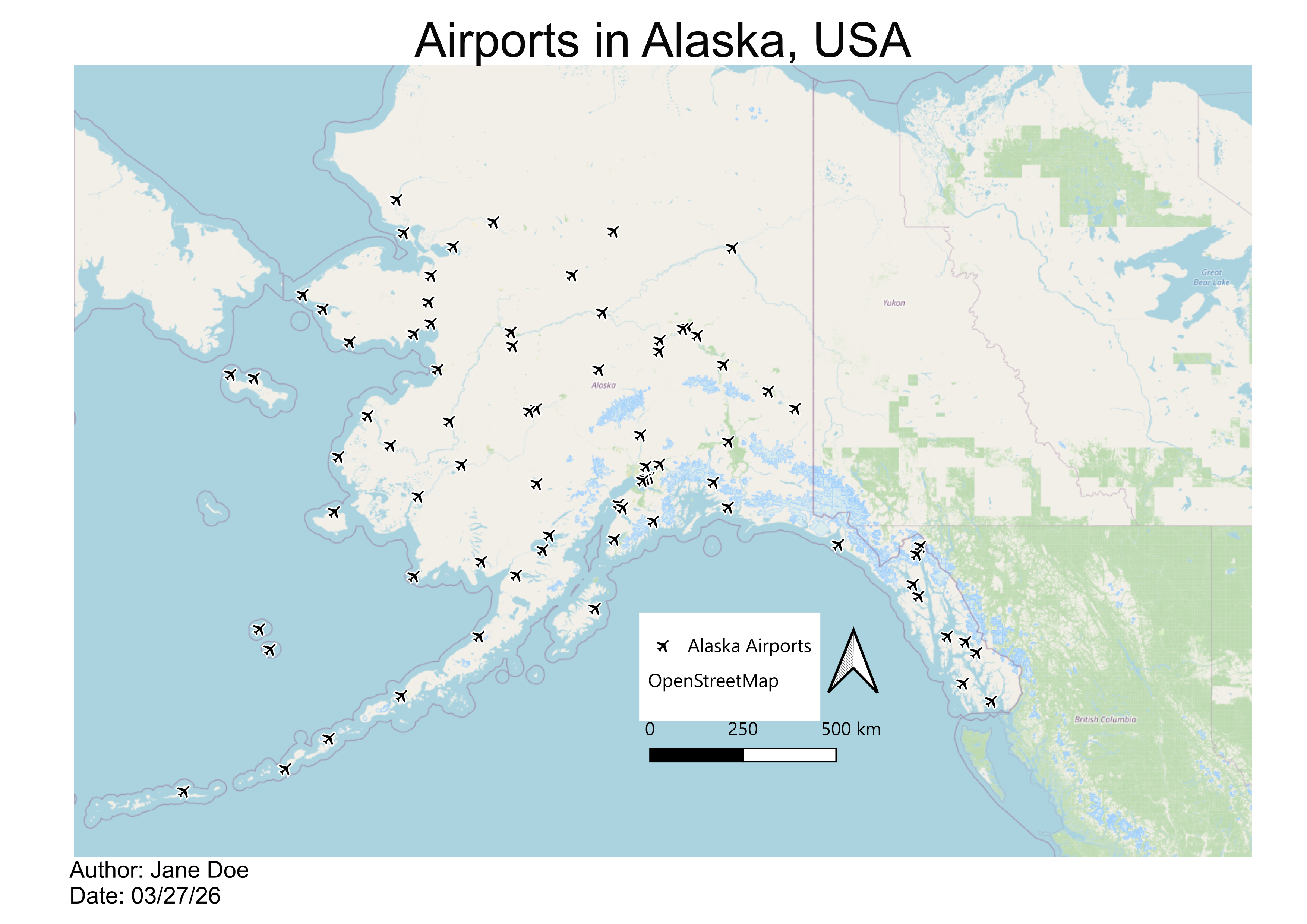
Below is an example of a finished map created using this workflow: Alaska airports displayed as point symbols over an OpenStreetMap basemap:
Common Beginner Mistakes
| Mistake | How to avoid it |
|---|---|
| Forgetting to save the project | Use Ctrl+S / Cmd+S frequently; save before every major step |
| Data layer hidden beneath the basemap | Check layer order in the Layers Panel; drag data layers above basemaps |
| Layer loaded but nothing appears on the map | Right-click the layer → Zoom to Layer |
| Shapefile won’t load | Ensure all five supporting files (.dbf,
.prj, .shx, .cpg) are in the same
folder as the .shp
|
| Legend shows code names instead of readable labels | Rename layers before building the layout via Properties → Source → Layer Name |
| Map exports blank | Make sure the layout’s map frame is linked to the correct map canvas |
| Overcomplicating symbology | Start with Single Symbol; add complexity only when it communicates something specific |
Exercise 1A.1: Guided Walkthrough
Load, Style, and Export Your First Map
Complete Parts 1 to 3 above using the QGIS sample airport dataset. By the end you should have:
- A QGIS project with an OpenStreetMap basemap and the airports shapefile loaded
- The airports layer styled with a symbol of your choice
- A Print Layout exported as a PDF or PNG that includes a title, legend, scale bar, north arrow, and data credit
Exercise 1A.2: Build a Multi-Layer Map of West Lafayette
Challenge
Real-world GIS projects rarely use a single data source. In this exercise you will combine three different data-loading methods (shapefiles, a geocoded CSV, and a live OpenStreetMap query) to build a multi-layer map.
Setup: Create a new QGIS project saved to your Session_1a folder.
Step 1: Download shapefiles from Natural Earth
Go to naturalearthdata.com and read the homepage briefly to understand the data’s purpose, scale, and reliability. Then navigate to Downloads → Medium Scale Data and download the following:
From Cultural:
- Admin-0 Country boundaries (polygon)
- Admin-1 States and Provinces (polygon)
- Populated Places (point)
From Physical:
- Rivers, Lake Centerlines (line)
Each download is a .zip file. Save them to your
Session_1a folder and unzip each one (as for the airports above), then
add them to your QGIS project using Layer → Add Layer → Add
Vector Layer (or drag the .shp files directly onto
the Layers Panel).
Step 2: Add point data from a CSV file
Download UFOreports_USonly_WorkshopLayer.csv from the
shared Session
1A Google folder and save it to your Session_1a folder. Then:
- Click the Open Data Source Manager button in the toolbar (or Layer → Data Source Manager).
- Select Delimited Text in the left panel.
- In the File Name field, navigate to the CSV file.
- Confirm that File Format is set to CSV.
- Verify that the X field and Y field are set to the longitude and latitude columns respectively, and that Geometry CRS is EPSG:4326 - WGS 84 (latitude and longitude in degrees).
- Click Add, then close the dialog.
This creates a temporary point layer. To keep it permanently, right-click the layer → Export → Save Features As… and save it as a shapefile or GeoPackage.
Step 3: Add live data via the QuickOSM plugin
OpenStreetMap contains a vast, continuously updated collection of mapped features. The QuickOSM plugin lets you query this data directly from within QGIS.
Install the plugin first:
- Go to Plugins → Manage and Install Plugins…
- Search for QuickOSM and click Install Plugin.
- While you have the plugin manager open, also install NextGIS QuickMapServices: this gives you access to a wider range of basemap options beyond OpenStreetMap.
Run a query:
- Go to Vector → QuickOSM → QuickOSM… and open the Quick query tab.
- In the Preset field, type
universityand select facilities/education/universities. - In the In field, type
West Lafayette, IN. - Click Run Query. A polygon layer for Purdue University’s campus should appear on your map.
- Right-click the new layer → Properties → Symbology to adjust its color and transparency.
Try a second query: repeat the process with shops/food
in the Preset field and the same location. This returns footprints for
food stores around Purdue’s campus.
Step 4: Style and build a map layout
Style each layer with a distinct color and adjust transparency as needed. Then turn off all layers except the Purdue campus polygon and the food stores layer. Open a new Print Layout and build a finished map that includes:
- A descriptive title
- A legend with readable layer names
- A scale bar
- A north arrow
- A data credit noting your name, data sources, and today’s date
Exercise 1A.3: Explore, Evaluate, and Map a Dataset of Your Choice
Challenge
Put your skills together using an external data source of your choosing. You can find a source in the previous episode here.
Part A: Choose and evaluate a dataset
Browse a public data repository and select a dataset that interests you. Before downloading:
- Read the source’s homepage or “About” page to understand its origin, coverage, and update frequency.
- Find and read the metadata. Note when it was last updated, how it was collected, what geographic area it covers, and what the key attribute fields represent.
- Write two to three sentences summarizing whether you think this dataset is reliable and appropriate for the kind of analysis you have in mind.
Part B: Download and add to QGIS
- Download your chosen dataset and save it to your Session_1a folder.
- Add it to your QGIS project using the appropriate method:
- Shapefile or GeoJSON → Layer → Add Vector Layer
- CSV with coordinates → Layer → Data Source Manager → Delimited Text
- Open the Attribute Table and explore the fields. Identify at least one field that could be used to style the layer with Graduated or Categorized symbology.
- Style the layer using that field.
Part C: Build a simple map layout
- Create a New Print Layout and add your styled layer.
- Include all required map elements: title, legend, scale bar, north arrow, and data credit.
- Export your map as a PNG or PDF.
Bonus: Find a second dataset on a related theme, add it as another layer, and adjust the symbology so both layers are visible and distinguishable.
Reflect on Your First Map
- What was the most confusing step in the workflow? How did you resolve it?
- Look at your finished map: what would you change to make it clearer for someone unfamiliar with the area?
- How does working with live OSM data (QuickOSM) differ from working with a downloaded shapefile? What are the trade-offs of each approach?