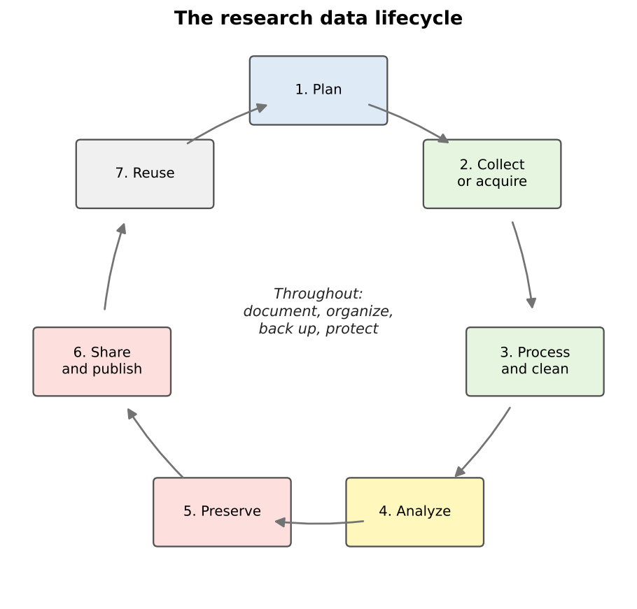
Image 1 of 1: ‘A cycle of seven boxes connected by arrows: 1 Plan, 2 Collect or acquire, 3 Process and clean, 4 Analyze, 5 Preserve, 6 Share and publish, 7 Reuse, which leads back to Plan. In the center: throughout, document, organize, back up, protect.’
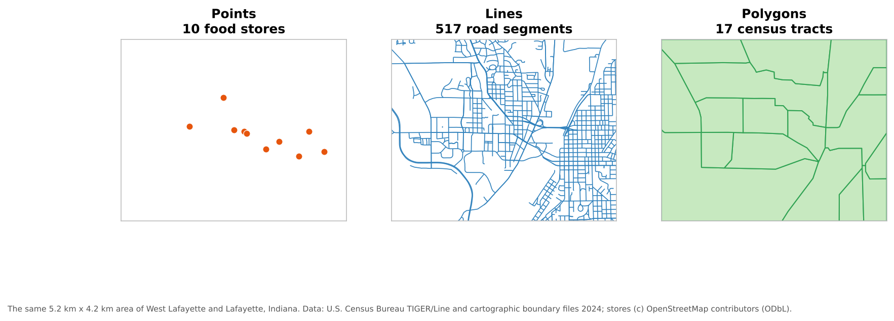
Image 1 of 1: ‘Three panels of the same area of West Lafayette and Lafayette, Indiana. Left, points: 10 orange dots for food stores. Middle, lines: a dense blue network of 517 road segments. Right, polygons: 17 green census tracts outlined in darker green.’
The three vector geometry types.
Figure 2
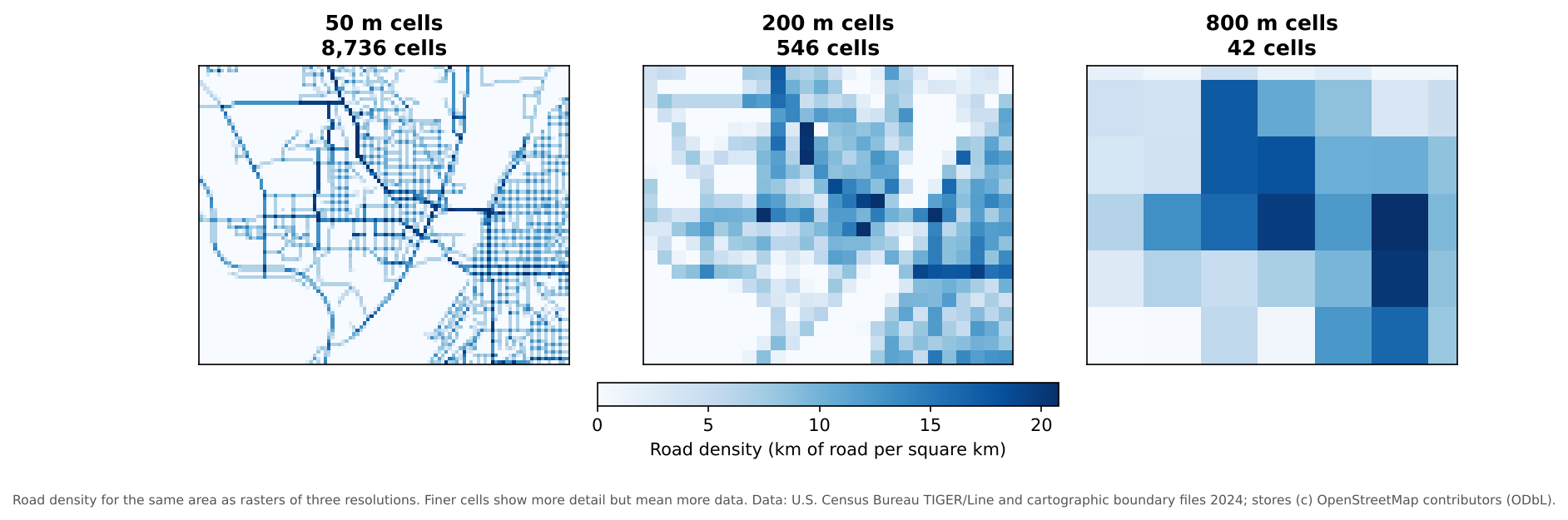
Image 1 of 1: ‘Three blue raster maps of road density for the same area. With 50 meter cells (8,736 cells) individual streets are visible. With 200 meter cells (546 cells) the pattern of dense neighborhoods is blocky but clear. With 800 meter cells (42 cells) only a coarse pattern remains.’
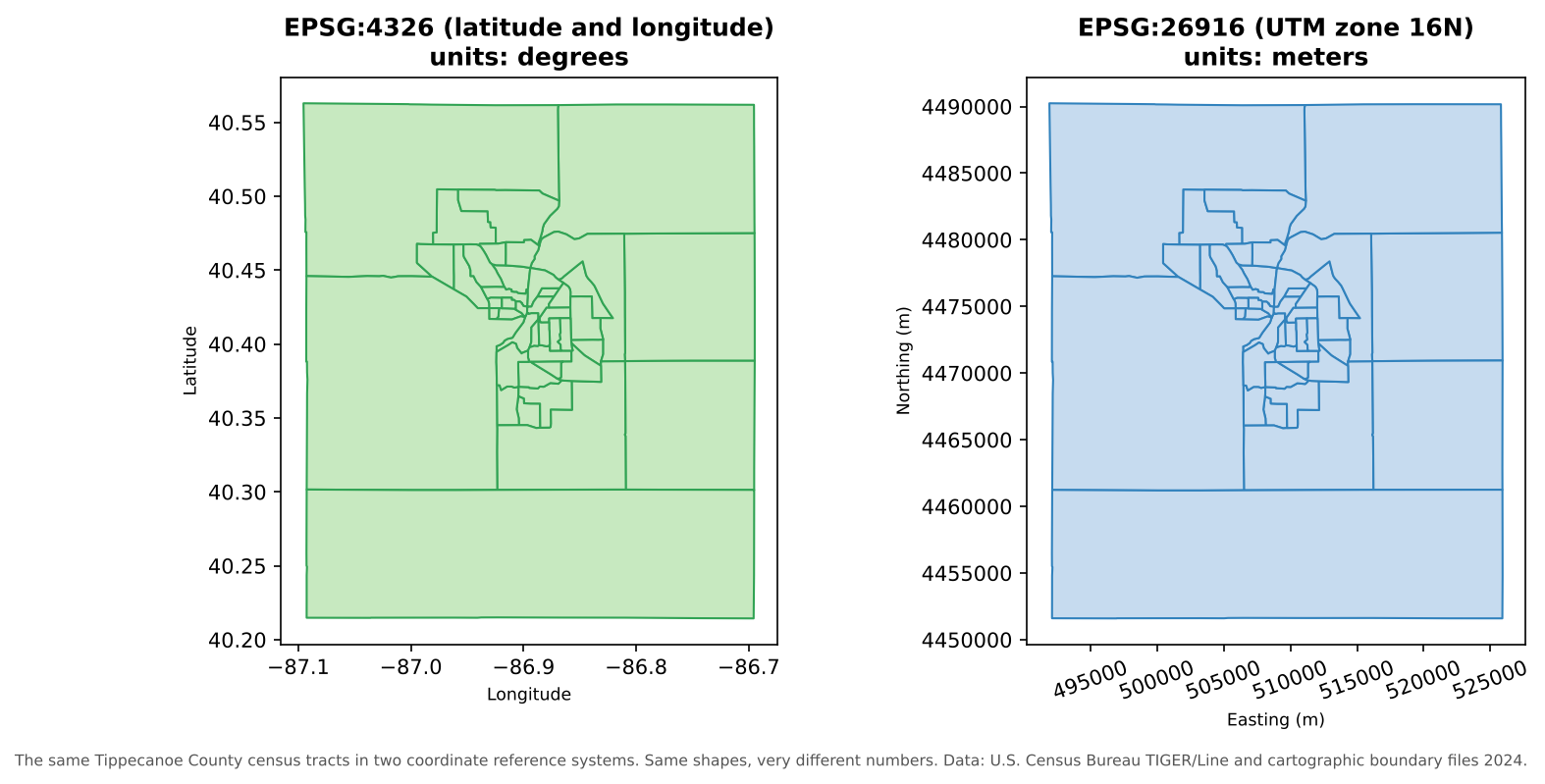
Image 1 of 1: ‘Two maps of the same Tippecanoe County census tracts. Left, in EPSG:4326, with axes in degrees: longitude from about -87.1 to -86.7 and latitude from about 40.2 to 40.55. Right, in EPSG:26916, with axes in meters: easting from about 492,000 to 526,000 and northing from about 4,451,000 to 4,490,000. The shapes look almost identical but the numbers are completely different.’
The same tracts in two coordinate reference
systems.
Image 1 of 1: ‘Four small diagrams. Gap between neighbors: two squares with a thin empty sliver between them, labeled gap. Overlapping polygons: two rectangles that overlap in a shaded strip, labeled overlap. Self-intersection: a bowtie-shaped polygon whose edges cross in the middle. Disconnected line: a vertical line that stops just short of a horizontal line, labeled undershoot, line stops short of the junction.’