All in One View

Content from Introduction to Data Management

Last updated on 2026-10-17 | Edit this page

Overview

Questions

What is research data management, and why does it matter for geospatial work?
What are the stages of the research data lifecycle?
What is a data management plan, and when is one required?

Objectives

Define research data management and distinguish it from data curation
Describe the stages of the research data lifecycle
List the main sections of a data management plan
Explain why geospatial data needs particular care

What is data management?

Research data management is everything you do to organize, store, protect and maintain data while a project is under way, so that the data stays usable, trustworthy and safe. It covers practical questions such as:

Where will the files live, and who can reach them?
What will the files and folders be called?
How will we know which version is the latest?
What happens if a laptop is lost or a hard drive fails?
How will someone else (or you, in a year) understand what each column means?

Good data management is not glamorous, but almost every researcher has a story of the alternative: a shapefile that no longer lines up, a folder of files called final_v3_REAL.shp, or a thesis chapter that could not be reproduced because the cleaned data was overwritten.

Management and curation

This module and the Data Curation module are closely related:

	Data management (this module)	Data curation
Focus	Day-to-day handling of data during a project	Making data understandable and usable beyond the project
Main tasks	Data models, formats, coordinate systems, organization, versions, backups, quality	Metadata, documentation, preservation, sharing, ethics
Main user	You and your team	Future users, including strangers and your future self

In practice they overlap, and both start on the first day of a project, not at the end.

The research data lifecycle

Data passes through stages that are often drawn as a cycle, because published data is reused to start new projects.

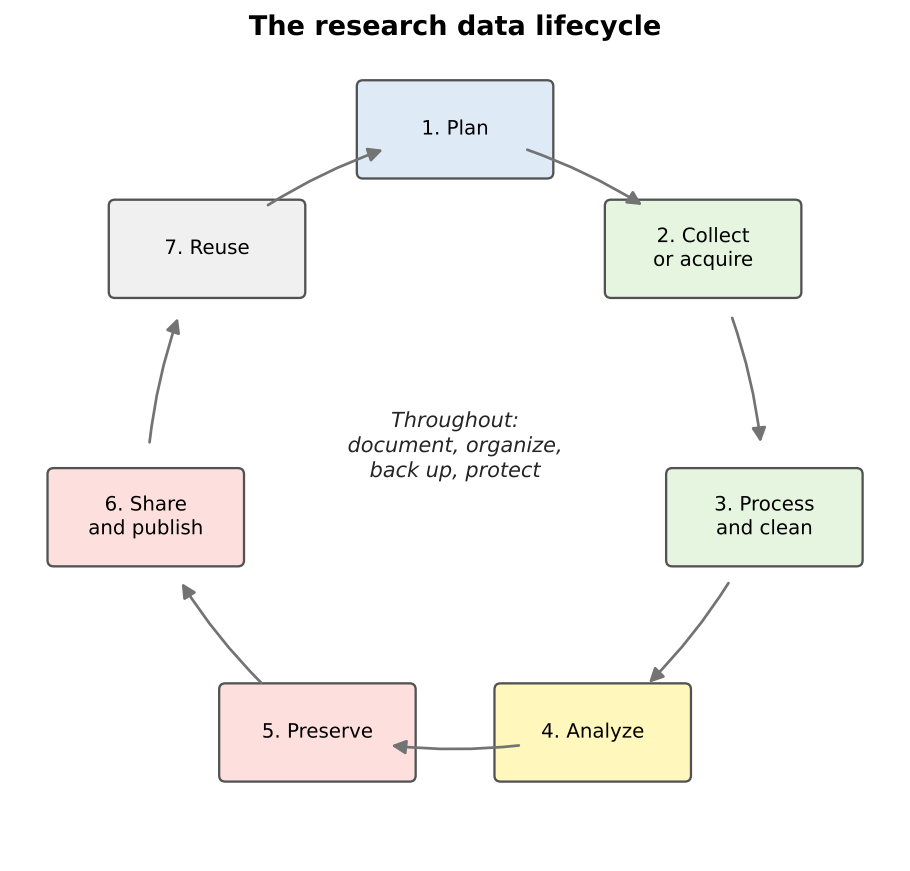
A cycle of seven boxes connected by arrows: 1 Plan, 2 Collect or acquire, 3 Process and clean, 4 Analyze, 5 Preserve, 6 Share and publish, 7 Reuse, which leads back to Plan. In the center: throughout, document, organize, back up, protect.

Stage	Geospatial example
Plan	Decide what layers you need, their coordinate system, file format and naming scheme
Collect or acquire	Download census tracts, digitize features from a scanned map, collect points with QField
Process and clean	Reproject layers, fix invalid geometries, join tables, remove duplicates
Analyze	Calculate distances, densities or statistics; make maps
Preserve	Save final datasets in stable, open formats with documentation
Share and publish	Deposit the data in a repository with a DOI and a license
Reuse	You, or others, start a new project from the published data

Some activities happen at every stage: documenting what you did, keeping files organized, backing them up, and protecting sensitive information.

Why geospatial data needs extra care

Geospatial data has all the problems of ordinary data, and a few of its own:

Many files make one dataset. A shapefile is at least three files that must travel together.
Coordinates mean nothing without a coordinate reference system. The same numbers can describe places hundreds of kilometers apart.
Data is often large. Imagery, elevation models and lidar can reach gigabytes or terabytes.
Geometry can be invalid in ways a spreadsheet never is: polygons that cross themselves, gaps between neighbors, lines that do not connect.
Location can be sensitive. A point can reveal where a person lives, works or receives care.
Software projects link to data by path. Move a folder and a QGIS project can lose its layers.

The rest of this module takes these one at a time.

Data management plans

A data management plan (DMP) is a short document, written before a project starts, that describes what data will be created and how it will be handled, shared and preserved. Many funders require one:

The U.S. National Science Foundation (NSF) requires a two-page Data Management and Sharing Plan with every proposal. If a project will not produce data, the proposal must explain why instead.
The National Institutes of Health (NIH) has required a Data Management and Sharing Plan for research that generates scientific data since January 2023.
A 2022 memorandum from the White House Office of Science and Technology Policy (the “Nelson memo”) directed federal agencies to make publications, and the data underlying them, publicly available without delay; agencies were asked to have updated policies in effect by the end of 2025.

Even when no funder asks for one, a DMP is a useful planning tool for a thesis or a team project.

What goes into a DMP

NSF’s guidance asks the plan to describe:

The data: what types of data, samples, software and other materials the project will produce
Standards: the formats and metadata standards that will be used
Access and sharing: how and when data will be shared, and how privacy, confidentiality, security and intellectual property will be protected
Reuse: policies for reuse, redistribution and derivative works
Archiving: how the data will be preserved and kept accessible

For a geospatial project, a good plan also names the coordinate reference system, the file formats, the expected data volume, and how any sensitive locations will be protected. Free tools such as DMPTool provide templates for each funder, and many university libraries (including Purdue’s) offer help writing plans.

Callout

Data management is a team responsibility

On a team project, decide early who is responsible for each task: who keeps the master copy, who approves changes to the schema, who checks backups. Write it down. “Everyone” usually means “no one”.

Challenge

Spot the risks

A graduate student keeps all of her thesis data in the Downloads folder of her laptop. Files have names such as tracts.shp, tracts2.shp, tracts_new.shp and export.csv. She sometimes edits the original census download directly. Name at least four risks, and a fix for each.

Show me the solution

No backup: if the laptop is lost or fails, everything is gone. Keep at least one other copy, ideally off-site or in institutional cloud storage.
Unclear names and versions: nobody can tell which tracts file is current or how they differ. Use descriptive names with dates or version numbers, and keep a short change log.
Raw data edited in place: the original can never be recovered. Keep raw data read-only and save changes as new files.
Disorganized location: the Downloads folder mixes project files with everything else. Use a dedicated project folder with a clear structure.
No documentation: there is no record of where export.csv came from or what its columns mean. Add a README and a data dictionary.

Challenge

Draft a mini plan

Pick a project you are working on, or imagine mapping grocery store access in your town. In five bullet points, one for each DMP section above, describe how you would manage the data.

Show me the solution

An example for a grocery access project:

Data: census tract boundaries and ACS tables (downloaded), grocery store points (field collected), road network (downloaded), maps and scripts.
Standards: GeoPackage for vector data, CSV for tables, EPSG:26916 for analysis, ISO 19115 metadata written in QGIS.
Access and sharing: store points shared openly after verification; no personal information collected.
Reuse: data released under a CC BY 4.0 license; OpenStreetMap-derived layers keep the ODbL.
Archiving: final datasets deposited in an institutional repository with a DOI.

Key Points

Data management is the day-to-day organization, storage, protection and maintenance of data during a project
The research data lifecycle runs from planning through collection, processing, analysis, preservation, sharing and reuse
Geospatial data needs extra care: multi-file formats, coordinate systems, large sizes, geometry validity and sensitive locations
Many funders, including NSF and NIH, require a data management and sharing plan, and a plan is worth writing even when not required

Content from Geospatial Data Models

Last updated on 2026-10-17 | Edit this page

Overview

Questions

How do computers represent places and features?
What are vector and raster data, and when should I use each?
How does map scale affect how a feature should be represented?

Objectives

Describe the three vector geometry types and how attributes are attached to them
Explain raster cells, resolution, bands and NoData values
Choose an appropriate data model and geometry for a research question
Explain what topology is and why it matters

Two ways to describe the world

A GIS has to turn a messy, continuous world into data a computer can store. There are two main approaches, called data models:

Vector: the world is made of discrete features (a store, a road, a county) with exact boundaries, each described by coordinates and a row of attributes.
Raster: the world is a surface divided into a grid of equal cells, and every cell holds a value (an elevation, a temperature, a land cover class, a color).

A third, very common kind of data is the plain table with no geometry at all, such as a spreadsheet of census counts. It becomes spatial when it is joined to a vector layer through a shared ID.

Vector data

Geometry

Vector features come in three basic geometry types:

Geometry	Stored as	Dimensions	Examples
Point	One x, y coordinate pair	None (a location)	Stores, wells, survey respondents, cell towers
Line (polyline)	An ordered list of points (vertices)	Length	Roads, rivers, transit routes, trails
Polygon	A closed ring of vertices, possibly with holes	Area and perimeter	Census tracts, parcels, lakes, building footprints

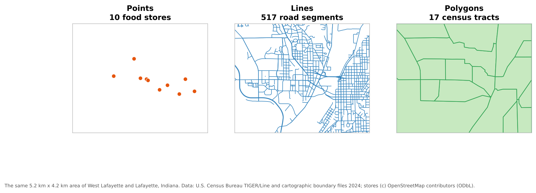
Three panels of the same area of West Lafayette and Lafayette, Indiana. Left, points: 10 orange dots for food stores. Middle, lines: a dense blue network of 517 road segments. Right, polygons: 17 green census tracts outlined in darker green.

There are also multi-part versions (a multipoint, a multiline, or a multipolygon such as Hawaii, which is one state made of several islands). Most file formats require all features in one layer to share the same geometry type, so stores, roads and tracts go in separate layers.

Attributes

Each feature has a row in an attribute table. The geometry says where; the attributes say what. A made-up example:

fid	store_name	store_type	snap_accepted	geometry
1	Example Supermarket	Supermarket	Yes	POINT (-86.9088 40.4539)
2	Example Market	Small market	Unknown	POINT (-86.9025 40.3863)
3	Example Corner Stop	Convenience	No	POINT (-86.8930 40.4190)

Designing those attributes well is the subject of the Designing Your Data episode.

Topology

Topology describes how features relate to each other: which polygons share a boundary, which lines meet at a junction, which point lies inside which polygon. Some data models store topology explicitly; most everyday formats (shapefile, GeoPackage, GeoJSON) store each feature independently and leave you to check that neighbors line up. Topology matters whenever the analysis depends on connections:

Network analysis needs road lines that actually meet at intersections
Neighboring census tracts should share boundaries exactly, with no gaps or overlaps
Each point should fall inside exactly one polygon of a zoning layer

The Data Quality episode shows common topology errors and how to find them.

Raster data

A raster is a grid of cells (or pixels), stored row by row. Its key properties are:

Property	Meaning	Example
Cell size (spatial resolution)	The ground width of one cell	10 m for Sentinel-2, 30 m for Landsat
Extent	The area the grid covers	One county, one satellite scene
Bands	Layers of values for the same cells	Red, green, blue and near-infrared bands of an image
Data type	What kind of number each cell holds	8-bit integers (0 to 255) for a photo; 32-bit decimals for temperature
NoData value	A special value meaning “no information here”	-9999, or areas outside the image

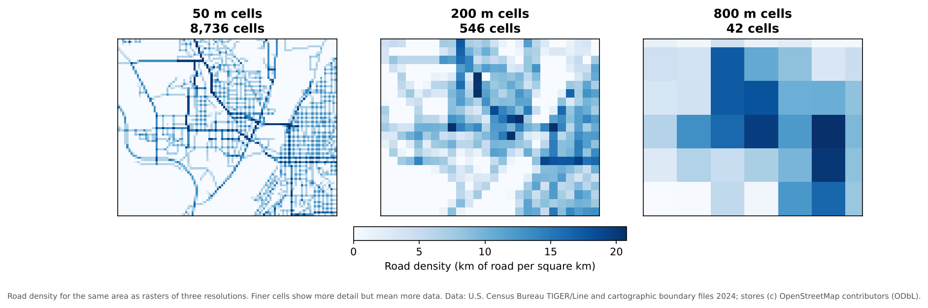
Three blue raster maps of road density for the same area. With 50 meter cells (8,736 cells) individual streets are visible. With 200 meter cells (546 cells) the pattern of dense neighborhoods is blocky but clear. With 800 meter cells (42 cells) only a coarse pattern remains.

Halving the cell size multiplies the number of cells by four, so resolution has a direct cost in storage and processing time. Choose the coarsest resolution that still answers your question.

Rasters come in two broad kinds:

Continuous rasters hold measured quantities that vary smoothly: elevation, temperature, rainfall, reflectance in a satellite band.
Categorical (discrete) rasters hold classes: land cover type, soil type, a zoning code. Their values are labels, so averaging them makes no sense.

Callout

NoData is not zero

A NoData cell means “unknown”, while 0 can be a real value (0 mm of rain, 0 m elevation at sea level). If the NoData value is not set correctly, a GIS will treat missing areas as real data and averages will be wrong. Always check a raster’s NoData value when you first open it.

Choosing a data model

Question	Usually best as
Where are the grocery stores, and what are they like?	Vector points
How long is the route to the nearest store?	Vector lines (a network)
How many households in each tract have no car?	Vector polygons joined to a table
How hot is each part of the city on a summer afternoon?	Raster (continuous)
What is the land cover around each school?	Raster (categorical), summarized to vector buffers

You can convert between models (rasterize vector data, or vectorize a raster), but every conversion loses something: rasterizing blurs exact boundaries to the cell size, and vectorizing a raster produces blocky, stair-stepped polygons.

Scale and generalization

How a feature should be represented depends on the scale of the map or analysis:

A city is a point on a map of the United States, but a polygon on a map of Indiana.
A river is a line on a state map, but a polygon (with two banks) on a detailed city map.
A building is a point in a regional study of businesses, but a polygon in a study of floor area.

Data made for small-scale maps is usually generalized: lines are simplified and small features dropped. The Census Bureau’s 1:20,000,000 cartographic boundary files are a good example. Generalized data looks fine on a national map but is not accurate enough for measuring distances or areas at the neighborhood level. Use data whose level of detail matches your analysis.

Challenge

Pick the model and geometry

How would you represent each of these, and why?

Bus stops in a city
Average annual rainfall across Indiana
School attendance zones
Hiking trails in a state park
Land cover (forest, farmland, urban, water) for a county

Show me the solution

Vector points: discrete locations with attributes such as routes served.
Raster (continuous): rainfall varies smoothly across space.
Vector polygons: each zone has a clear boundary and attributes such as school name.
Vector lines: trails have length and connect at junctions; topology matters for routing.
Raster (categorical): land cover is usually classified from satellite imagery, cell by cell. It can be converted to polygons for some uses, at the cost of blocky edges.

Challenge

Resolution and storage

A single-band raster covering a 50 km by 50 km county has 30 m cells and stores each cell in 4 bytes. About how large is it? What happens if you switch to 10 m cells?

Show me the solution

50,000 m / 30 m is about 1,667 cells on each side, or about 2.8 million cells. At 4 bytes each, that is about 11 MB. With 10 m cells there are 5,000 cells per side, or 25 million cells, about 100 MB: nine times larger, because resolution improved three times in both directions. Multi-band images multiply this again by the number of bands.

Key Points

Vector data represents discrete features as points, lines or polygons, each with a row of attributes
Raster data represents surfaces as a grid of cells with a resolution, bands, a data type and a NoData value
Topology describes how features connect and share boundaries; network and boundary analysis depend on it
The right data model and geometry depend on the question and the scale of the analysis
Finer raster resolution grows data size with the square of the change in cell size

Content from Geospatial File Formats

Last updated on 2026-10-17 | Edit this page

Overview

Questions

What are the common file formats for vector and raster data?
What are the limitations of the shapefile?
Which format should I use to work with, to share, and to archive my data?

Objectives

Recognize the most common vector and raster file formats and their file extensions
Explain the strengths and limitations of shapefiles, GeoPackages and GeoJSON
Distinguish open from proprietary formats
Choose a suitable format for working, sharing and long-term storage

Why formats matter

The same map layer can be stored in many file formats. The choice affects whether others can open your data, whether attribute names and values survive, how large the files are, and whether the data will still be readable in twenty years. A few questions to ask of any format:

Is it open (a published, freely implementable specification) or proprietary (controlled by one company)?
Is it one file or several that must stay together?
Does it preserve the coordinate reference system, field names, data types and null values?
How large can it get, and how fast is it?

Vector formats

Format	Extension(s)	Open?	Notes
Shapefile	`.shp` `.shx` `.dbf` `.prj` (and others)	Published by Esri	The old standard; widely supported but limited (see below)
GeoPackage	`.gpkg`	Yes (OGC standard)	One file holding many vector layers, tables and even rasters; the default in QGIS
GeoJSON	`.geojson`	Yes (IETF RFC 7946)	Plain text; ideal for the web and small datasets; always in longitude and latitude (WGS 84)
KML / KMZ	`.kml` `.kmz`	Yes (OGC standard)	Google Earth’s format; good for sharing with the public, weak for analysis
CSV with coordinates	`.csv`	Yes	A table with x and y (or longitude and latitude) columns; only points; the CRS must be documented separately
File geodatabase	`.gdb` (a folder)	No (Esri)	ArcGIS’s main format; readable by QGIS and GDAL, but best kept for ArcGIS workflows
GeoParquet	`.parquet`	Yes (open specification, version 1.1)	Columnar format for large datasets and cloud analysis; growing quickly

The trouble with shapefiles

The shapefile dates from the early 1990s. It is everywhere, and every GIS can read it, but it has real limitations:

Several files make one dataset. At minimum .shp (geometry), .shx (index) and .dbf (attributes); usually also .prj (coordinate system) and .cpg (text encoding). Lose the .prj and the layer no longer knows where it is; lose the .dbf and the attributes are gone.
Field names are limited to 10 characters. produce_available becomes produce_av, and two long names can collide.
Text fields hold at most 254 characters, and there is no true date-and-time type.
Each file is limited to 2 GB.
One geometry type per file, and no way to store several layers together.
Null values are poorly supported, so missing numbers often turn into 0.

None of these are a problem for a quick download, but they cause silent data loss when you save your own carefully designed data as a shapefile.

Callout

Prefer GeoPackage for your own work

A GeoPackage is a single file (an SQLite database) that can hold all the layers of a project, with long field names, real date and time fields, proper null values and no 2 GB limit. It is an Open Geospatial Consortium (OGC) standard and the default format in QGIS. If you receive shapefiles, it is good practice to convert them to a GeoPackage at the start of a project.

Raster formats

Format	Extension(s)	Notes
GeoTIFF	`.tif` `.tiff`	The standard raster format: a TIFF image with georeferencing built in; supports many bands and data types
Cloud Optimized GeoTIFF (COG)	`.tif`	A GeoTIFF organized so programs can read just the part they need over the web; an OGC standard
JPEG 2000	`.jp2`	Compressed imagery; used by Sentinel-2
NetCDF and HDF5	`.nc` `.h5`	Multidimensional arrays (for example, temperature by latitude, longitude, height and time); common for climate and Earth observation data
Zarr	a folder	A cloud-friendly format for very large multidimensional arrays
ASCII grid	`.asc`	A plain-text grid; easy to read, but large and slow
PNG or JPEG with a world file	`.png` + `.pgw`	An ordinary image plus a small text file of georeferencing; fine for display, not for analysis

Compression

Raster files can be compressed to save space. Lossless compression (such as DEFLATE or LZW in a GeoTIFF) keeps every value exactly. Lossy compression (such as JPEG) discards detail to save more space, which is acceptable for a background image but not for data you will measure or analyze.

Tables

Tables without geometry are often the largest part of a social science project. CSV is the safest format for sharing them: it is plain text, opens anywhere, and will remain readable for decades. Spreadsheet files (.xlsx) are convenient for editing but can hide problems: merged cells, formulas, colors that carry meaning, and automatic conversion of codes such as 01001 into the number 1001 or of MAR1 into a date.

Callout

Watch out for leading zeros

FIPS codes and GEOIDs often start with zero (01 is Alabama, 01001 is Autauga County). Opening a CSV in a spreadsheet program can silently turn them into numbers and drop the zero, breaking every later join. Import ID columns as text, and check them after every conversion.

Which format when?

Purpose	Good choices	Why
Working copy of a project	GeoPackage (vector), GeoTIFF (raster)	Complete, fast, few limitations
Sharing with collaborators	GeoPackage, or the format they use	One file is easy to send
Web maps and small datasets	GeoJSON	Readable by web libraries and by people
Very large vector data	GeoParquet	Fast, compact, cloud-friendly
Large imagery shared online	Cloud Optimized GeoTIFF	Readers can fetch only what they need
Long-term preservation	Open, well-documented formats: GeoPackage, GeoJSON, GeoTIFF, CSV	Readable without any one company’s software

Converting between formats

Conversions are routine (in QGIS, right-click a layer and choose Export > Save Features As…), but each one is a chance to lose information. After converting, check:

that the coordinate reference system is still correct
that field names were not shortened and data types did not change (text IDs becoming numbers)
that null values did not become 0 or empty strings
that the number of features is the same
that special characters (accents, non-Latin scripts) display correctly

Behind most GIS software, including QGIS, is the open-source GDAL library, which reads and writes more than 200 formats. That is why QGIS can open almost anything you are given.

Challenge

What went wrong?

A colleague sends you a zip file containing stores.shp and stores.dbf. When you open it in QGIS, the points appear near the coast of Africa, and a field called produce_av holds values that should be in produce_available. What happened, and what would you ask for?

Show me the solution

The .prj file is missing, so QGIS does not know the layer’s coordinate reference system. The points are probably in a projected system (with coordinates in meters) being read as degrees, or in degrees being read as the wrong system, so they land near 0° latitude, 0° longitude. The .shx index is also missing, which some software cannot do without. The shortened field name is the shapefile’s 10-character limit. Ask for the complete set of files (including .shx and .prj), or better, a GeoPackage, plus the CRS (for example its EPSG code).

Challenge

Choose a format

What format would you use for each, and why?

A field team’s grocery store points, with long field names and a date and time for each visit
A small layer of 20 campus buildings for an interactive web map
A 40 GB set of Landsat images to share with collaborators who will analyze small areas
A table of ACS estimates by census tract that will be archived with a thesis

Show me the solution

GeoPackage: long field names, true date and time fields and proper nulls; a shapefile would truncate names and lose the times.
GeoJSON: small, plain text, and read directly by web mapping libraries.
Cloud Optimized GeoTIFF: collaborators can read only the areas they need instead of downloading 40 GB.
CSV, with GEOIDs stored as text and a data dictionary describing each column: open, simple and durable.

Key Points

Formats differ in openness, number of files, size limits and what attribute information they preserve
Shapefiles are universal but limited: several files, 10-character field names, 2 GB, weak null support
GeoPackage is a good default for your own vector work; GeoTIFF for rasters; CSV for tables
Prefer open, well-documented formats for sharing and preservation
Check the CRS, field names, data types, nulls and feature counts after every conversion

Content from Coordinate Reference Systems

Last updated on 2026-10-17 | Edit this page

Overview

Questions

What is a coordinate reference system, and why does every layer need one?
What is the difference between geographic and projected coordinate systems?
What are EPSG codes, and which ones will I meet most often?
Why do layers sometimes appear in the wrong place, and how do I fix it?

Objectives

Explain the parts of a coordinate reference system: datum, coordinate system and units
Distinguish geographic from projected coordinate systems and know when to use each
Recognize common EPSG codes for work in the United States
Distinguish defining a coordinate system from reprojecting data, and avoid the classic mistakes

Coordinates need context

The numbers 507575, 4474900 and -86.9107, 40.4247 describe the same place: the Purdue Memorial Union. The first pair is in meters in one system; the second is in degrees in another. Coordinates only mean something together with their coordinate reference system (CRS), which says how the numbers relate to locations on Earth.

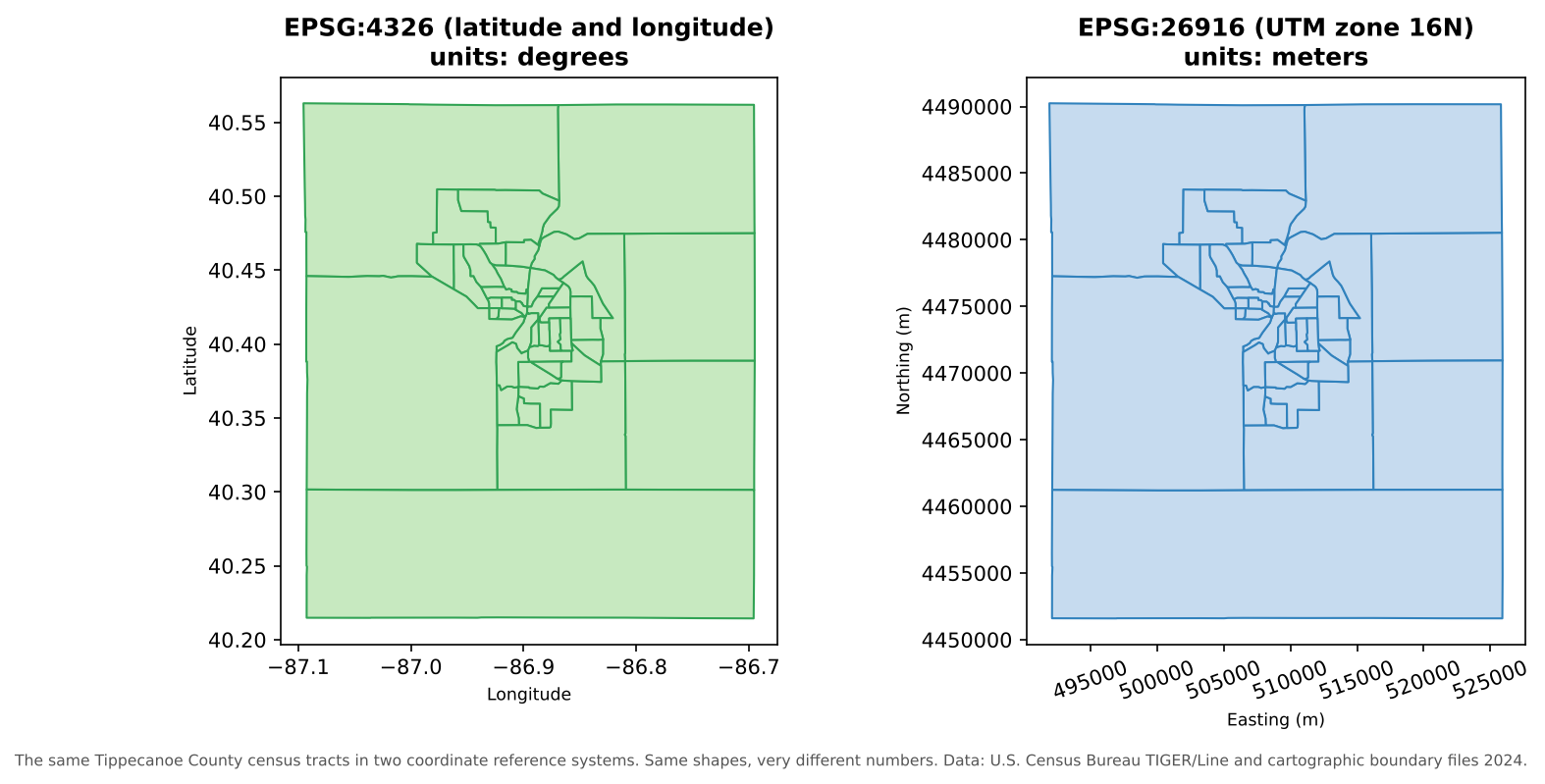
Two maps of the same Tippecanoe County census tracts. Left, in EPSG:4326, with axes in degrees: longitude from about -87.1 to -86.7 and latitude from about 40.2 to 40.55. Right, in EPSG:26916, with axes in meters: easting from about 492,000 to 526,000 and northing from about 4,451,000 to 4,490,000. The shapes look almost identical but the numbers are completely different.

Managing the CRS of every layer is one of the most important, and most often neglected, parts of managing geospatial data.

The parts of a CRS

Part	What it does	Examples
Datum	A model of the Earth’s shape (an ellipsoid) and how it is anchored to the real Earth	WGS 84 (used by GPS), NAD83 (the official datum for North America)
Coordinate system	How positions are expressed: angles on the ellipsoid, or x and y on a flat projection	Latitude and longitude; UTM easting and northing
Units	The units of the coordinates	Degrees, meters, U.S. survey feet
Projection (projected systems only)	The mathematical method for flattening the curved Earth	Transverse Mercator, Albers Equal Area, Lambert Conformal Conic

Different datums place the same point at slightly different coordinates. In the contiguous United States, NAD83 and WGS 84 differ by about one to two meters: irrelevant for a state map, but important for surveying or precise field data.

Geographic and projected systems

	Geographic CRS	Projected CRS
Coordinates	Latitude and longitude	x (easting) and y (northing)
Units	Degrees	Usually meters or feet
Shape of Earth	Curved (a 3D ellipsoid)	Flat (a 2D plane)
Good for	Storing and exchanging data, global datasets, GPS	Measuring distances and areas, analysis, local mapping
Example	EPSG:4326 (WGS 84)	EPSG:26916 (NAD83 / UTM zone 16N)

A degree of longitude is about 111 km at the equator but only about 85 km in Indiana, and it shrinks to zero at the poles. So distances and areas calculated in degrees are meaningless. Before measuring anything, reproject to a suitable projected CRS.

Every projection distorts something: area, shape, distance or direction. Choose one that preserves what your analysis needs:

Equal-area projections (such as Albers) for comparing areas and densities across a large region
Conformal projections (such as UTM or Lambert Conformal Conic) for local shapes and angles
UTM zones and State Plane zones for accurate local measurements

Choosing a projection for a finished map, and seeing how projections distort the world, is covered in the Data Visualization module’s Fundamentals of Map Design episode.

EPSG codes

Every common CRS has a numeric code in the EPSG registry (originally compiled by the European Petroleum Survey Group). Using codes avoids ambiguity: “UTM” alone is not enough, but EPSG:26916 is exact.

EPSG code	Name	Use
4326	WGS 84 (latitude and longitude)	GPS, GeoJSON, most web data, global datasets
4269	NAD83 (latitude and longitude)	U.S. federal data, including Census TIGER/Line files
3857	WGS 84 / Pseudo-Mercator	Web map tiles (Google, OpenStreetMap, Esri). For display only: areas are badly distorted
5070	NAD83 / Conus Albers	Equal-area maps and analysis of the contiguous United States
26916	NAD83 / UTM zone 16N	Accurate local measurement in Indiana and neighboring states
32616	WGS 84 / UTM zone 16N	The same zone on the WGS 84 datum

You can look up any code, and find the right one for an area, at https://epsg.io/.

How the CRS is stored

In a shapefile, the CRS is in the separate .prj file.
In a GeoPackage or GeoTIFF, it is stored inside the file.
GeoJSON (RFC 7946) is always in WGS 84 longitude and latitude.
A CSV of coordinates stores no CRS at all: you must document it, for example in a column name (lon_wgs84) and in the README.

Defining versus reprojecting

These two operations sound similar but do very different things:

	Defining (assigning) a CRS	Reprojecting (transforming)
What it does	Tells the software which CRS the coordinates are already in	Calculates new coordinates in a different CRS
Changes the numbers?	No	Yes
When to use	The CRS is missing or wrong, and you know the correct one	You need the data in another CRS for analysis or to match other layers
In QGIS	Layer Properties > Source > Assigned Coordinate Reference System, or the Assign projection tool	Reproject layer tool, or Export > Save Features As… with a new CRS

The classic mistake is to define a CRS when you meant to reproject. The numbers stay the same, but the software now believes they mean something else, and the layer jumps to the wrong place (or the wrong continent).

Callout

On-the-fly reprojection can hide problems

QGIS reprojects every layer on the fly to the project’s CRS, so layers in different systems still draw in the right place. That is convenient, but it can hide the fact that your layers differ. Tools that combine layers (clip, join by location, distance and network tools) work best, and sometimes only work correctly, when the layers share one projected CRS. Some tools also report results in the project’s units. Before analysis, reproject every layer to the same projected CRS and set the project to it.

Troubleshooting checklist

Symptom	Likely cause	Fix
Layer appears near 0° latitude, 0° longitude (off West Africa)	Projected coordinates (meters) read as degrees, or a missing CRS	Find the correct CRS and define it
Layer is shifted by a meter or two	Datum mismatch (for example NAD27 and NAD83, or NAD83 and WGS 84 with no transformation)	Use the right datum transformation when reprojecting
Areas or distances are tiny numbers such as 0.0002	Calculated in degrees	Reproject to a projected CRS first
Areas look far too large near the poles	Calculated in Web Mercator (EPSG:3857)	Use an equal-area projection
Layer will not appear at all	Coordinates in the wrong order (latitude, longitude swapped)	Check which column is x and which is y

Challenge

Define or reproject?

For each situation, should you define (assign) the CRS or reproject the data?

You receive a shapefile with no .prj, and the metadata says the data is in NAD83 / UTM zone 16N.
Your census tracts are in NAD83 latitude and longitude, and you need to calculate their areas in square kilometers.
Your field points were collected in WGS 84, and the rest of the project is in EPSG:26916.

Show me the solution

Define EPSG:26916. The coordinates are already in that system; the software just does not know it.
Reproject to an equal-area projected CRS (such as EPSG:5070) or a local one (EPSG:26916), then calculate areas.
Reproject the points to EPSG:26916 so every layer shares one projected CRS.

Challenge

Read the coordinates

Without opening a GIS, which CRS is each of these coordinate pairs probably in?

(-86.91, 40.42)
(507575, 4474900)
(-9675000, 4928000)

Show me the solution

Geographic (latitude and longitude, such as EPSG:4326 or 4269): small numbers within -180 to 180 and -90 to 90.
UTM (here zone 16N): eastings around 500,000 m and northings in the millions of meters.
Web Mercator (EPSG:3857): coordinates in meters from the equator and the prime meridian, with large negative x values in the Western Hemisphere.

Key Points

Coordinates are meaningless without their coordinate reference system: datum, coordinate system, units and projection
Store and exchange data in geographic systems; measure and analyze in projected ones
Use EPSG codes to name CRSs exactly; 4326, 4269, 3857, 5070 and 26916 are common in U.S. work
Defining a CRS labels existing coordinates; reprojecting calculates new ones. Confusing the two moves data to the wrong place
Before analysis, put every layer, and the project, in the same projected CRS

Content from Designing Your Data

Last updated on 2026-10-17 | Edit this page

Overview

Questions

How do I decide what layers and attributes a project needs?
What is a data dictionary, and what goes in it?
How do field types, domains and unique IDs keep data consistent?
How do tables relate to each other and to map layers?

Objectives

Translate a research question into layers, geometries and attributes
Write a data dictionary with field names, types, lengths, domains and null rules
Explain the role of primary keys and foreign keys in joining data
Recognize one-to-one, one-to-many and many-to-many relationships

Start from the question

Designing a dataset (sometimes called schema design or, in a GIS, geodatabase design) is the most important and most time-consuming part of building one. Decisions made here are hard to change later, after hundreds of records have been entered. Work through these steps on paper or in a spreadsheet before creating anything in a GIS.

Step 1: What things will you record?

List each kind of object or phenomenon you will record. Each usually becomes its own layer (or table). For a study of food access, these might be grocery stores, bus stops, and survey respondents’ neighborhoods.

Step 2: What geometry suits each one?

Decide whether each is best represented as a point, line or polygon at the scale you will analyze it (see the Geospatial Data Models episode). A store is a point for an access study but could be a polygon for a study of store size.

Step 3: What do you need to know about each one?

Brainstorm the attributes: the questions you will ask of the data. For grocery stores:

Type of information	Example attributes
Identity of the store	store ID, name, chain or brand
Location	address, city, ZIP code, coordinates
Benefits accepted	SNAP accepted, WIC accepted
Food available	fresh produce available, fresh meat available
When it was observed	date and time of the visit, hours posted
Anything else relevant	notes
Evidence	storefront photograph

Only collect what you will use. Every extra field costs time to collect and check, and personal information creates obligations to protect it.

The data dictionary

A data dictionary turns that list into precise fields. It is both a design tool and a key piece of documentation: it tells everyone who enters or uses the data exactly what each field means.

Data dictionary for the grocery store point layer
Field name	Description	Type	Length	Allowed values (domain)	Nulls allowed?
`store_id`	Unique ID for each store	Integer		Assigned automatically, never reused	No
`store_name`	Name shown on the store’s sign	Text	60	Free text	No
`store_type`	Kind of store	Text	20	Supermarket, Small market, Convenience, Other	No
`address`	Street address	Text	80	Free text	Yes
`city`	City	Text	30	Lafayette, West Lafayette, Other	No
`zip`	ZIP code	Text	5	Five digits	Yes
`snap_accepted`	SNAP benefits accepted, based on posted signs	Text	7	Yes, No, Unknown	No
`wic_accepted`	WIC benefits accepted, based on posted signs	Text	7	Yes, No, Unknown	No
`produce_available`	Fresh produce on sale at the visit	Text	7	Yes, No, Unknown	No
`visit_datetime`	Date and time of the field visit	Date and time			No
`hours_posted`	Opening hours as posted on the door	Text	100	Free text	Yes
`notes`	Anything unusual about the visit	Text	250	Free text	Yes
`photo`	Storefront photograph	Attachment (file path)			Yes

Field types

Choose the type that matches how the value will be used:

Type	Use for	Watch out for
Integer	Counts and ID numbers you will calculate with	Not for codes with leading zeros
Decimal (real, double)	Measurements: distances, percentages, prices	Set enough precision
Text (string)	Names, categories, and codes such as ZIP codes and GEOIDs	Set a sensible maximum length
Date and date and time	When something happened	Shapefiles cannot store times; use GeoPackage
Boolean (true or false)	Simple yes or no	Cannot say “unknown”; a Yes, No, Unknown text domain is often better

A useful rule: if you would never do arithmetic with it, store it as text. ZIP codes, FIPS codes, GEOIDs and phone numbers are labels, not quantities.

Domains

A domain is the list (or range) of values a field may hold. Dropdown menus in a field app enforce it. Domains prevent the most common data entry problem: the same thing written many ways (“SNAP”, “snap”, “EBT”, “yes”). In QGIS, domains are set in Layer Properties > Attributes Form with the Value Map widget; in a GeoPackage or file geodatabase they can also be stored in the data itself.

Include Unknown in categorical domains. A blank can mean “unknown”, “not applicable” or “forgot to fill in”; an explicit Unknown is honest and unambiguous.

Field names

Good field names are:

short but meaningful: snap_accepted, not snap or does_the_store_accept_snap_benefits
lowercase with underscores, no spaces or special characters, and not starting with a number
consistent: if one field is wic_accepted, the next is snap_accepted, not SNAPaccept
10 characters or fewer only if the data must ever be saved as a shapefile

Unique IDs and keys

Every feature needs a unique identifier that never changes and is never reused. Names make poor IDs: two stores can share a name, and names change. Coordinates make poor IDs too, because they change when a point is corrected.

In database terms:

A primary key uniquely identifies each row of a table (store_id in the store layer; GEOID in a census tract layer).
A foreign key is a field in another table that refers to a primary key (a store_id column in a table of repeated visits; a GEOID column in a table of ACS estimates).

Joins work by matching keys, so keys must have identical values and types in both tables. A GEOID stored as text in one table and as a number in the other will not match.

Relationships between tables

Relationship	Example	How to handle it
One-to-one	Each census tract has one row of ACS estimates	A simple join adds the columns to the tract layer
One-to-many	Each store is visited several times	Keep visits in a separate table with a `store_id` foreign key, and link it with a relation rather than copying store details into every visit
Many-to-many	Stores accept many benefit programs; each program is accepted by many stores	Use a third linking table with one row per store and program

Keeping repeated information in separate, linked tables (called normalization) avoids inconsistencies: if a store’s name is stored once, it cannot be spelled two different ways. QGIS supports this through Project Properties > Relations, and a GeoPackage can hold all the linked tables in one file.

Callout

Some choices are easy to change later, some are not

Adding a new field later is easy. Renaming fields, changing a field’s type, changing the geometry type, or changing the meaning of a category after data has been collected is hard and error-prone. Spend the time on the design, test it on a few real records, and only then start collecting.

Challenge

Fix the data dictionary

What is wrong with each of these field definitions, and how would you fix it?

Field name	Type	Allowed values
`Store Name`	Text
`zip`	Integer
`open`	Boolean	true, false
`type`	Text	free text

Show me the solution

Store Name contains a space and capitals; use store_name.
zip as an integer drops leading zeros (02134 becomes 2134) and invites meaningless arithmetic; store it as text with a length of 5.
open is ambiguous (open now? open 24 hours?) and a Boolean cannot say “unknown”. Use a clearer name, such as open_at_visit, with a Yes, No, Unknown domain.
type as free text will produce inconsistent categories; give it a domain such as Supermarket, Small market, Convenience, Other. A more specific name (store_type) also helps.

Challenge

Design your own

Choose a topic from your own research or teaching (for example, park amenities, public art, or vacant lots). Write a data dictionary with at least six fields, including a unique ID, at least two fields with domains, and a date field. Decide which fields may be null.

Show me the solution

Answers will vary. Check your design against these questions:

Does every feature get a unique, permanent ID?
Do categorical fields have domains that include Unknown?
Are codes stored as text and measurements as numbers?
Are field names short, lowercase and free of spaces?
Is there a date (and time, if it matters) for when each record was observed?
Does every field have a description someone else could understand?

Key Points

Design data from the research question: the things you record become layers, and the questions become attributes
A data dictionary defines each field’s name, meaning, type, length, allowed values and null rule
Store codes such as ZIP codes and GEOIDs as text; use domains with an Unknown option for categories
Every feature needs a permanent unique ID; joins match primary keys to foreign keys
Keep repeated information in separate related tables rather than copying it

Content from Organizing, Versioning and Backing Up

Last updated on 2026-10-17 | Edit this page

Overview

Questions

How should I organize the folders of a geospatial project?
What makes a good file name?
How do I keep track of versions without losing work?
How should I store and back up my data?

Objectives

Set up a clear project folder structure that separates raw, processed and output data
Apply file naming conventions that sort well and work on every computer
Keep QGIS projects portable with relative paths
Choose a versioning approach and apply the 3-2-1 backup rule

A place for everything

A consistent folder structure means you, your collaborators and your future self can find things without asking. One widely used layout for a geospatial project:

grocery_access_2026/
├── README.md                  what the project is, who made it, how the folders are organized
├── data/
│   ├── raw/                   original downloads and field exports; never edited
│   ├── processed/             cleaned, reprojected and joined data
│   └── documentation/         data dictionaries, metadata, source notes
├── scripts/                   Python or R code, numbered in the order they run
├── qgis/                      QGIS project files (.qgz) and saved styles
├── outputs/
│   ├── maps/                  exported map images and PDFs
│   └── tables/                summary tables and statistics
└── docs/                      reports, presentations and the thesis or paper

The details can vary, but three principles matter most:

Raw data is read-only. Keep the original download or field export exactly as you received it, and never edit it. Every change produces a new file in processed/. If something goes wrong, you can always start again from the original. (On most systems you can mark the folder or files as read-only.)
Separate inputs, processing and outputs. Anyone should be able to tell what came from elsewhere, what you made, and what you are presenting.
Document the structure in a README at the top of the project.

File naming

Good file names are descriptive, consistent and machine-friendly.

Instead of	Use	Why
`final_FINAL_v2 (copy).shp`	`tippecanoe_tracts_2024_utm16n.gpkg`	Says what, where, when and in which CRS
`Tracts New.gpkg`	`tracts_new.gpkg`	No spaces or capitals; works in every program and in scripts
`map 3-4-26.png`	`2026-03-04_no_car_households_map.png`	ISO 8601 dates (YYYY-MM-DD) sort in date order
`data.csv`	`acs2024_tippecanoe_tracts_b08201.csv`	Unique and self-explanatory even outside its folder
`clean.py`, `analysis.py`	`01_download.py`, `02_clean.py`, `03_analysis.py`	Numbers show the order to run them

Rules of thumb:

Use only letters, numbers, underscores (_) and hyphens (-). Avoid spaces and characters such as & % # ( ) ' /.
Put the most important element first, so related files sort together.
Write dates as YYYY-MM-DD (or YYYYMMDD).
Pad numbers with zeros (01, 02, … 10) so they sort correctly.
Agree on the convention with your team and write it in the README.

Keep QGIS projects portable

A QGIS project file (.qgz) does not contain the data; it stores paths to each layer. If those paths are absolute (C:\Users\Maria\Desktop\project\data\roads.gpkg), the project breaks as soon as the folder is moved, renamed or opened on another computer.

Use relative paths (../data/processed/roads.gpkg). In QGIS this is the default, set in Project > Properties > General > Save paths.
Keep data inside the project folder rather than scattered across the computer.
If layers break, QGIS opens a Handle Unavailable Layers dialog where you can point each layer to its new location.

Version control

Data and code change constantly during a project. Without a system, you end up with a folder of near-identical files and no idea which one is current.

Simple versioning

For small projects, a clear manual system works:

Add a version number or date to processed files: stores_v01.gpkg, stores_v02.gpkg, or stores_2026-03-04.gpkg.
Keep a change log (a plain text file) that records what changed in each version and why:

2026-03-04  stores_v02.gpkg  Removed 2 duplicate stores (Fresh Foods, Main St.); fixed 5 store_type values.
2026-02-20  stores_v01.gpkg  First cleaned version of the field export.

Never reuse a version number, and never edit an old version.

Git and GitHub

Git is a version control system that records every change to a set of files, who made it and why, and lets you return to any earlier state. GitHub hosts Git repositories online for sharing and collaboration (these lessons are themselves Git repositories on GitHub).

Git is excellent for code, documentation and small text-based data such as CSV and GeoJSON files, where it can show exactly which lines changed. It is a poor fit for large binary files (imagery, large GeoPackages): it cannot show what changed inside them, and repositories grow quickly. GitHub warns about files larger than 50 MB and blocks files larger than 100 MB. Large data is better kept in research storage or a data repository, with only the code and documentation in Git.

Storage and backup

Where to keep the working copy

Option	Good for	Watch out for
Your laptop	Fast day-to-day work	Theft, loss, hardware failure
External drive	A local backup copy	Easy to lose; drives fail; keep it in a different place
Institutional cloud or research storage	Collaboration and secure, backed-up storage	Check what kinds of data your institution allows there
Commercial cloud storage	Convenient syncing	Data protection rules; syncing also spreads accidental deletions

Universities provide approved storage for research data; at Purdue, Research Computing and the Libraries can advise on the right option for a project. Sensitive data (for example, data about identifiable people) may only be stored in approved, secure locations.

Callout

Syncing is not backup

A synced folder copies your mistakes too: delete or overwrite a file and the change reaches every copy within seconds. A backup is a separate copy, ideally with older versions kept, that you can restore from.

The 3-2-1 rule

Keep at least:

3 copies of your data (the working copy plus two backups),
on 2 different types of storage (for example, your laptop and a cloud service),
with 1 copy off-site (in a different building, or in the cloud).

And test your backups: a backup you have never restored from is a hope, not a plan.

Challenge

Rename these files

Rewrite each name following the conventions in this episode:

Final Map (2).png, a map of grocery stores made on 7 March 2026
tracts.shp, Indiana census tracts for 2024 in UTM zone 16N
New Microsoft Excel Worksheet.xlsx, ACS vehicle data for Tippecanoe County tracts
script.py, the second script in the workflow, which joins ACS data to tracts

Show me the solution

2026-03-07_grocery_stores_map.png
indiana_tracts_2024_utm16n.gpkg (also converting it to a GeoPackage)
acs2024_tippecanoe_tracts_vehicles.csv (as CSV for a durable, open copy)
02_join_acs_to_tracts.py

Challenge

Is this backed up?

A researcher keeps her project on her laptop, in a folder synced to a cloud service. Does she meet the 3-2-1 rule? What could still go wrong?

Show me the solution

Not quite. She has two copies on two kinds of storage, one of them off-site, but syncing means an accidental deletion, overwrite or ransomware infection on the laptop is copied to the cloud. She needs a third, separate copy, for example a scheduled backup to an external drive or a backup service that keeps older versions. Checking that the cloud service keeps version history (and for how long) would also help.

Key Points

Use a consistent folder structure that separates raw, processed and output data, and keep raw data read-only
Name files descriptively and consistently, without spaces, with ISO 8601 dates and zero-padded numbers
Keep data inside the project folder and use relative paths so QGIS projects stay portable
Track versions with numbered files and a change log, or with Git for code and small text data
Follow the 3-2-1 backup rule, remember that syncing is not backup, and test your backups

Content from Data Quality

Last updated on 2026-10-17 | Edit this page

Overview

Questions

What does “quality” mean for geospatial data?
What kinds of errors are common in vector data?
How can I check and improve the quality of a dataset?

Objectives

Describe the elements of spatial data quality
Recognize invalid geometries and topology errors
Plan a quality assurance and quality control workflow
Record quality checks so others can judge fitness for use

Quality means “fit for use”

No dataset is perfect. A road layer accurate to 10 meters is excellent for a regional access study and useless for engineering a new intersection. Data quality is therefore about fitness for use: is the data good enough for this purpose, and do we know its limitations?

The elements of spatial data quality

International standard ISO 19157 (endorsed by the U.S. Federal Geographic Data Committee) describes data quality through a set of elements. In plain terms:

Element	Question	Grocery store example
Completeness	Is anything missing (omission) or extra (commission)?	A new store is missing; a closed store is still listed
Logical consistency	Does the data follow its own rules: domains, formats, topology?	`store_type` contains “gas station”, which is not in the domain
Positional accuracy	How close are the coordinates to the true location?	A point is 40 m from the store, in the parking lot
Thematic (attribute) accuracy	Are the attribute values correct? Are the classes right?	A store marked as accepting SNAP does not
Temporal quality	Is the data current, and are dates correct and consistent?	Hours were recorded three years ago
Usability	Overall, can it be used for the intended purpose?	Good enough for a city-wide access study?

A further, essential piece of information is lineage: where the data came from and what was done to it. Without lineage, nobody can judge the other elements. (Lineage is recorded in metadata; see the Data Curation module.)

Geometry errors

Vector geometry has rules. A polygon’s boundary must close and must not cross itself; neighboring polygons in a layer such as census tracts should not overlap or leave gaps. Data that breaks these rules can make tools fail or, worse, quietly give wrong answers.

Four small diagrams. Gap between neighbors: two squares with a thin empty sliver between them, labeled gap. Overlapping polygons: two rectangles that overlap in a shaded strip, labeled overlap. Self-intersection: a bowtie-shaped polygon whose edges cross in the middle. Disconnected line: a vertical line that stops just short of a horizontal line, labeled undershoot, line stops short of the junction.

Error	What it is	Typical cause	Why it matters
Invalid geometry (for example a self-intersection)	A polygon whose edges cross, or a ring that does not close	Careless digitizing, format conversion	Overlay, clip and area tools fail or return nonsense
Gaps and slivers	Thin empty spaces between polygons that should touch	Digitizing neighbors separately; mixing data of different scales	Points in the gap belong to no polygon; totals do not add up
Overlaps	Two polygons covering the same area	The same causes	Areas and counts are double-counted
Undershoots and overshoots (dangles)	Lines that stop short of, or cross past, the line they should meet	Digitizing without snapping	Network routes break or go the wrong way
Duplicate features	The same feature entered twice	Repeated imports; several data collectors	Counts and access measures are inflated
Null or empty geometry	A record with no shape	Failed edits or imports	The feature silently disappears from maps and analyses

Finding and fixing them in QGIS

QGIS has tools in the Processing Toolbox for each kind of problem:

Check validity (Vector geometry group) lists invalid geometries and explains each error
Fix geometries creates a repaired copy of a layer (always keep the original)
The Check geometry group includes tools such as Small gaps, Overlaps, Self-intersections, Dangle-end lines and Duplicated geometries
Delete duplicate geometries and Delete duplicates by attribute remove exact copies
Snapping options (Project > Snapping Options) prevent undershoots and gaps while you digitize

Automatic fixes are a starting point, not an answer. Look at what was changed before trusting it.

Attribute errors

Problems in the attribute table are at least as common as geometry problems:

values outside the domain (misspellings, inconsistent capitalization, old categories)
impossible values (a negative population, a store opening at 25:00, a percentage over 100)
missing values, and missing values disguised as 0 or -9999
IDs that are not unique, or that lost their leading zeros
units mixed within a column (miles and kilometers, dollars and thousands of dollars)

Simple checks catch most of them: count the distinct values in each categorical field, look at the minimum and maximum of each numeric field, and count nulls. In QGIS, Vector > Analysis Tools > Basic Statistics for Fields and the Statistics panel do this quickly.

Quality assurance and quality control

Quality assurance (QA) prevents errors: a careful design, domains and dropdowns, required fields, snapping, training, and a test run before collecting.
Quality control (QC) finds errors afterwards: validity and topology checks, attribute summaries, comparisons with another source, and field checks of a sample.

A practical QC routine for each new or updated dataset:

Confirm the CRS and that the layer lines up with a trusted reference layer.
Count features, and compare with what you expect.
Run Check validity and the relevant Check geometry tools.
Summarize each attribute: distinct values, ranges and nulls.
Look for duplicates by ID, by name and by location.
Check a random sample against a reference (imagery, a website, a field visit).
Record what you checked, what you found and what you changed.

Callout

Report quality honestly

Every dataset has limitations. State them: “Store locations were collected with phone GPS (typically 3 to 10 m accuracy); 12 of 64 stores were verified in the field in March 2026.” This kind of statement does not weaken your work. It lets others use your data correctly, and it is part of good metadata.

Challenge

Name the quality element

Which element of data quality does each problem affect?

A census tract layer is from 2010, but the analysis is about 2024.
Three stores were recorded twice by different volunteers.
A store’s point is on the wrong side of a river.
store_type contains the values “Supermarket”, “supermarket” and “Grocery”.
Two new supermarkets that opened last year are missing.

Show me the solution

Temporal quality (tract boundaries were redrawn for 2020)
Completeness (commission: extra records), and logical consistency if IDs are duplicated
Positional accuracy
Logical consistency (values outside the domain), and thematic accuracy if “Grocery” is a different category
Completeness (omission)

Challenge

Why did the total change?

A researcher sums the population of all tracts that intersect a city and gets a number 4% higher than the city’s official population. Give two possible data quality explanations.

Show me the solution

Overlaps: if some tract polygons overlap, people are counted twice.
Mismatched geometry: tracts that only touch or slightly cross the city boundary (because of slivers or boundaries digitized at different scales) are included in full, adding people who live outside the city.
Temporal mismatch: the tract populations and the official city figure may describe different years.

Checking overlaps, using tract centroids (or proper areal weighting) instead of “intersects”, and matching years would resolve it.

Key Points

Data quality means fitness for a particular use, and every dataset has limitations
The elements of quality are completeness, logical consistency, positional accuracy, thematic accuracy and temporal quality, with lineage recorded alongside
Invalid geometries, gaps, overlaps, dangles and duplicates are common vector errors; QGIS has tools to find each
Prevent errors with good design (QA) and find them with systematic checks (QC)
Record what you checked and report limitations honestly