Tables, Joins and Selections in QGIS

Overview

Questions

• How do I attach a table of statistics to map features in QGIS?
• Why do ID columns cause so many failed joins?
• How do I calculate rates, and what happens with zeros and missing values?
• How do I select and export the features that meet a condition?

Objectives

• Load a CSV table from the web and inspect field types
• Join a Census table to census tracts with a table join, and check that it worked
• Create rate fields with the Field Calculator and handle division by zero and Census “no estimate” codes
• Select features by expression, summarize them, and export the result

Why tables matter

---

Most social science data arrives as a table: a spreadsheet of counts by county, tract or ZIP code, with no shapes in it. To map it, you attach it to boundaries that share an ID. This is the most common task in applied GIS, and also the most common place for silent mistakes.

This episode uses Tippecanoe County, Indiana (Lafayette and West Lafayette):

Dataset	File	Contents
Census tracts (polygons)	tippecanoe_tracts.geojson	43 tracts with GEOID, name and land area aland_m2
ACS 2024 table (no shapes)	tippecanoe_acs_2024.csv	One row per tract: GEOID, total_pop, pop_under18, median_income, poverty_universe, below_poverty, households, hh_no_vehicle

Web addresses to copy:

• Census tracts (polygons): https://raw.githubusercontent.com/SpatialTurn/Foundations/main/data/tippecanoe_tracts.geojson
• ACS 2024 table (no shapes): https://raw.githubusercontent.com/SpatialTurn/Foundations/main/data/tippecanoe_acs_2024.csv

The table holds 2024 American Community Survey (ACS) 5-year estimates, downloaded once from the Census API for this lesson. The Data Collection module’s Census episode shows how to request them yourself. The same steps in Python are in Foundations notebooks 3a (tables) and 4c (joins).

IDs, types and joins

---

A table join (also called an attribute join) adds the columns of a table to the features of a layer wherever an ID matches. Census data uses GEOIDs, built by concatenating codes:

Part	Digits	Tippecanoe example
State	2	18 (Indiana)
County	3	157 (Tippecanoe)
Tract	6	010400
Tract GEOID	11	18157010400

A GEOID looks like a number but is really a code, and it should be stored as text. Alabama’s state code is 01, so an Alabama tract GEOID such as 01001020100 loses its leading zero if a program reads it as a number (1001020100), and it will never match the text version in the boundary file. Every field has a type (text, integer, decimal, date), and QGIS shows it next to the field name. Checking types before a join saves hours.

After every join, check two things:

1. Did every feature find a match? Count the features whose joined columns are empty (NULL).
2. Did any feature match twice? A table with duplicate IDs can make a join pick an arbitrary row.

Rates, zeros and missing values

---

Counts mostly show where many people live. To compare tracts, divide by the right denominator:

Rate	Numerator	Denominator
Households without a vehicle (%)	hh_no_vehicle	households
Below the poverty line (%)	below_poverty	poverty_universe (people whose poverty status is known)
Children (%)	pop_under18	total_pop

Two kinds of trouble appear in real Census tables:

• Zero denominators. Census Tract 104 holds Purdue’s residence halls: 8,248 people but 0 households and a poverty universe of 0, because people in group quarters (dorms, prisons, nursing homes) are not households and are excluded from poverty counts. Dividing by zero has no answer; QGIS returns NULL, which is correct, and the tract should be shown as “no data”, not as 0%.
• Special codes. Where the Census cannot produce an estimate it puts a code instead of a value. Median income is -666666666 for tracts 104 and 105. If you leave it in, any average or map of income is ruined. Replace codes with NULL before using the field.

Student populations also explain why tracts near campus show very high poverty rates: students often report low incomes while being supported by family or loans. That is a real feature of the data, not an error, but it must be explained in any map of poverty in a college town.

---

Hands-on

---

These steps were checked in QGIS 4.0 (QGIS 3.34 and later are nearly identical).

Part 1: Load the layer and the table

1. Load the tracts web address with Layer > Add Layer > Add Vector Layer, Source Type: Protocol: HTTP(S), cloud, etc., Type: HTTP/HTTPS/FTP, as in the previous episode.
2. Load the ACS table web address the same way. A CSV without coordinates loads as a table: it appears in the Layers panel with a table icon and draws nothing on the map.

Check: 43 tract polygons over Tippecanoe County, and a tippecanoe_acs_2024 table in the Layers panel.

Part 2: Look at the table and its field types

1. Right-click tippecanoe_acs_2024 and choose Open Attribute Table. Sort by total_pop by clicking its header. Find tracts 104 and 105 and look at households and median_income.
2. Close the table. Right-click the table again, choose Properties > Fields. The Type column shows GEOID and name as String (text) and the counts as Integer.
3. Do the same for the tracts layer: its GEOID is also String. The two ID fields match in type, so the join will work.

Check: both GEOID fields are String, and tract 104 has 0 households.

Callout

How did QGIS know the types?

A CSV file is plain text and does not store types. This one comes with a small companion file, tippecanoe_acs_2024.csvt, that lists them, and QGIS reads it automatically. Without it, QGIS would read every column as text when loading from the web, or guess the types when you load a downloaded CSV with Layer > Add Layer > Add Delimited Text Layer. That dialog guesses GEOID is a number unless you tell it otherwise, which is exactly how leading zeros get lost in states whose codes start with 0.

Part 3: Join the table to the tracts

1. Right-click the tracts layer, choose Properties, then the Joins tab.
2. Click the green + button at the bottom.
3. Join layer: tippecanoe_acs_2024. Join field: GEOID. Target field: GEOID.
4. Leave Custom field name prefix as it is (tippecanoe_acs_2024_) or shorten it to acs_. This episode uses acs_.
5. Click OK. The join appears in the list; click the arrow next to it to see its settings.

The Joins tab of the tracts layer’s properties, with the join to the ACS table.

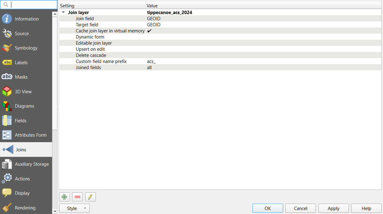
6. Click OK again to close the Properties.

Check: open the tracts’ attribute table. New columns such as acs_total_pop and acs_households appear at the right, filled in for every row.

To check for unmatched features properly, use an expression:

1. In the tracts’ attribute table, click Select features using an expression (the icon with an epsilon and a yellow square).
2. Enter "acs_total_pop" IS NULL and click Select Features.

Check: the title bar of the table says 0 selected. If it says 43, the join failed completely; look again at the ID fields and their types.

A table join is virtual: the CSV is not copied into the tracts file, and the columns are looked up each time. Part 6 shows how to save the result as a new file.

Part 4: Calculate rates with the Field Calculator

The tracts layer came from the web, so it is read-only. We add virtual fields: calculated columns stored in the project rather than in the data file, which suits read-only and joined layers.

1. In the tracts’ attribute table, click the Field Calculator (the abacus icon).

2. Create virtual field is already ticked and grayed out, with a note at the bottom: “This layer does not support adding new provider fields. You can only add virtual fields.” That is expected for a layer read from the web. Output field name: pct_no_vehicle. Output field type: Decimal (double).

3. Expression:

   "acs_hh_no_vehicle" / "acs_households" * 100

4. Look at the Preview under the expression, then click OK.

The Field Calculator creating a virtual field.

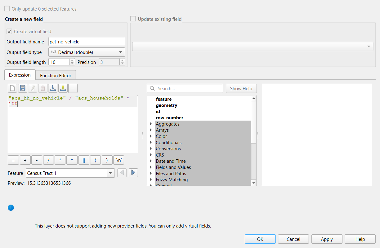
Check: a new pct_no_vehicle column. Sort it: the highest values (above 30%) are tracts 105, 55 and 4, and tract 104 shows NULL because it has no households.

Now clean the income field. Create another virtual field, income, type Integer (32 bit), with:

if("acs_median_income" < 0, NULL, "acs_median_income")

if(condition, value if true, value if false) is one of the most useful expressions in QGIS: here, any negative code becomes NULL and real values pass through.

Check: income is NULL for tracts 104 and 105, and the lowest real value is about $12,600.

Part 5: Select by expression and summarize

1. Open Select features using an expression again (or Edit > Select > Select Features by Expression).
2. Enter "pct_no_vehicle" >= 10 and click Select Features, then Close.
3. The selected tracts turn yellow on the map. Right-click the layer and choose Zoom to Selection if you like.
4. Open View > Panels > Statistics, choose the tracts layer and the field acs_hh_no_vehicle, and tick Selected features only.

Check: 17 tracts are selected. The Statistics panel shows their total households without a vehicle.

Selecting is different from filtering: a selection highlights features but keeps everything in the layer, while Filter… (right-click the layer) hides everything that does not match until you clear it.

Part 6: Save the joined result

1. Right-click the tracts layer and choose Export > Save Features As…
2. Format: GeoPackage. File name: browse to your project folder and name it tippecanoe_tracts_acs.
3. Tick Save only selected features if you want just the 17 tracts; leave it unticked for all 43.
4. Click OK. The new layer is added to the map.

Check: open the new layer’s attribute table. The joined acs_ columns and your virtual fields are now real columns in the file.

---

Challenge

Challenge 1: Poverty rate

Create a virtual field poverty_rate with the share of people below the poverty line. Which tract has the highest rate, and which tract cannot have one?

Show me the solution

Expression: "acs_below_poverty" / "acs_poverty_universe" * 100. The highest is Census Tract 105 (about 80%), followed by tracts 54.02, 55 and 112, all near Purdue’s campus, where many residents are students. Tract 104 has a poverty universe of 0 (residence halls), so its rate is NULL.

Challenge

Challenge 2: Why did the join fail?

A colleague joins a county table to Alabama county boundaries on GEOID. Every joined field is NULL. In the table, GEOID shows values like 1001; in the boundaries, 01001. What happened, and how can it be fixed in QGIS?

Show me the solution

The table’s GEOID was read as a number, which dropped the leading zero, so 1001 never matches the text 01001. Fixes, from best to quickest:

• Reload the CSV and set the field type to text (in the Delimited Text dialog, Custom field types, or with a .csvt file).
• Or create a text field in the table with the Field Calculator, lpad(to_string("GEOID"), 5, '0'), and join on it instead.

Then check again for NULLs.

Challenge

Challenge 3: Count or rate?

You want to show where households without a car are concentrated, to plan a grocery delivery service. Should the map show acs_hh_no_vehicle or pct_no_vehicle? Discuss.

Show me the solution

It depends on the question. For planning a service, the count matters: a large tract with 5% carless households may contain more households to serve than a small tract with 30%. For comparing need or inequality between neighborhoods, the rate is fair because it removes the effect of tract size. A good choropleth uses the rate; counts are better shown with graduated symbols (circles sized by count). Many reports show both.

Key Points

• A table join attaches a table to features by a shared ID; check that ID fields have the same type first
• Census GEOIDs are codes: store them as text so leading zeros survive
• After a join, select "field" IS NULL to find unmatched features
• Rates need the right denominator; division by zero gives NULL, and Census codes such as -666666666 must be replaced with NULL
• Selection highlights features, Filter hides the others, and Save Features As makes joins and virtual fields permanent