
All in One View
Content from Exercises: Acquiring Raster Data using Imagery Databases
Last updated on 2026-06-28 | Edit this page
Estimated time: 55 minutes
Overview
Questions
- Where can I find scanned historical maps for use in GIS?
- What is CORONA satellite imagery and how do I download it?
- How do I acquire Sentinel-2 multispectral imagery?
- What is a digital elevation model (DEM) and where do I get one?
Objectives
- Understand the difference between georeferenced and non-georeferenced raster data
- Download a scanned historical map from a public repository
- Search for and download CORONA imagery from the CAST website and USGS EarthExplorer
- Download Sentinel-2 imagery from the Copernicus Browser
- Download SRTM elevation data from USGS EarthExplorer
Introduction
Raster data — scanned maps, aerial photographs, satellite imagery, elevation models — forms the visual backbone of many GIS projects. Some raster files come georeferenced (positioned in real-world coordinates and ready to use), while others, like scanned paper maps, are non-georeferenced and must be aligned manually before they can overlay with other data layers.
This session covers four types of raster data, moving from historical sources to modern satellite products.
1. Scanned Historical Maps
Several public and academic websites host scanned paper maps that are free to download. These are typically non-georeferenced — you will need to georeference them before using them in QGIS.
Useful Map Repositories
- Perry-Castañeda Library Map Collection — University of Texas; thousands of scanned maps organized by region
- National Library of Australia Trove — Australian maps, photographs, and archival material
- Old Maps Online — aggregates historical maps from libraries worldwide
Walkthrough: Perry-Castañeda Library
- Go to https://legacy.lib.utexas.edu/maps/
- Scroll down and click Historical
- Browse by topic or region until you find a useful map — large military topographic series often include index maps to help locate a specific area
- Right-click the map image and select Save Image As, then save it to your project folder
2. CORONA Satellite Imagery
During the Cold War the United States operated a series of classified reconnaissance satellites. The CORONA program (1960–1972) produced over 860,000 black-and-white images — the first high-resolution (up to ~2 m) stereo photographs of the Earth’s surface. The imagery was declassified in 1995.
The highest-resolution images come from the KH-4B series (1967–1972), captured on panoramic film strips each covering roughly 8.6 × 117 km. High-resolution scans are available from USGS EarthExplorer at no cost (at up to 3600 dpi), or for $30 per frame for scenes that have not yet been scanned.
Since declassification, CORONA imagery has been widely used to study historical landscapes, identify archaeological sites, trace old land tenure boundaries, and document features lost to urbanization or agricultural expansion.
Option A: Pre-Georeferenced Imagery from CAST
The CORONA Atlas at the University of Arkansas CAST provides a subset of CORONA scenes that have already been georeferenced — ready to use directly in QGIS.
- Go to https://corona.cast.uark.edu/ and click Explore Atlas
- Red rectangles on the map show available missions — zoom in to your area of interest
- Use the slider tool at the bottom of the screen to compare CORONA and modern imagery side by side
- Adjust transparency with the slider next to Corona Imagery to see how features have changed
- Expand the Corona Imagery layer with the (+) button to see individual images
Tip
As you zoom in, fewer missions will be listed — this is normal, since each scene covers a specific footprint.
- Toggle images on and off to find the best one, then click the blue download button (V) next to it
- Click Download GeoTiff — these are large files, so the download may take a few minutes
- Move the downloaded file to a dedicated folder (e.g.,
CORONA/) in your GIS project directory
Loading the image in QGIS
- Open QGIS and click the Open Data Source Manager button on the toolbar
- Select the Raster tab, click Browse, and navigate to your CORONA GeoTIFF
- Click Open → Add → Close
Exercise 1: Download from CAST
Download a CORONA image of your area of interest (or a famous landmark) from the CAST website. Load it into QGIS and explore the scene.
Option B: Full Archive from USGS EarthExplorer
The CAST atlas covers a limited area. For global coverage, use the complete CORONA archive on USGS EarthExplorer.
Before You Begin
Make sure you are logged in to your EarthExplorer account. If you do not have one, create a free account at https://earthexplorer.usgs.gov/.
Step 1: Define Your Search Area
- In the map window, navigate to your area of interest
- Click corners on the map to draw a search polygon, or zoom in and click Use Map in the Search Criteria pane
- Your search area will appear as a semi-transparent red polygon
Step 2: Select the Dataset
- Click the Data Sets tab
- Expand Declassified Data → select Declass 1 (1996)
Step 3: Filter for High-Quality Imagery
- Click the Additional Criteria tab
- Expand Camera Resolution and select Stereo High (this limits results to the best KH-4B imagery)
- Optionally, expand Download Availability and select Yes to show only pre-scanned images (leave blank to see all coverage, including frames available for $30)
Step 4: Review and Download
- Click Results to see available scenes
- Use the Footprint and Image Overlay icons to preview coverage on the map
- Click Show Metadata and Browse (the paper icon) to check cloud cover and image clarity
- When you have chosen a scene, click the Download Options button (disk icon with green arrow) and select Download
Step 5: Extract the Files
- Move the downloaded
.tgzfile to your project folder - Extract with 7-Zip → Extract Here to get a
.tarfile - Extract the
.tarfile again — this produces four.tiffiles (the panoramic strip split into segments labeled a, b, c, and d)
Note
Raw CORONA imagery from EarthExplorer is not georeferenced. You will need to georeference it in QGIS before it can be overlaid with other spatial data.
3. Sentinel-2 Multispectral Imagery
The Sentinel-2 satellite program, launched in 2015 by the European Space Agency as part of the EU’s Copernicus programme, provides free, high-resolution multispectral imagery across 13 spectral bands. Two satellites (2A and 2B) image the entire land surface approximately every 5 days at 10 m resolution in the visible bands.
Sentinel-2 imagery is especially useful for land cover classification, vegetation health monitoring (NDVI), and environmental change detection.
Searching and Downloading from the Copernicus Browser
Before You Begin
Make sure you have a Copernicus Data Space account. Register for free at https://identity.dataspace.copernicus.eu/.
- Log in and navigate to the Copernicus Browser
- Zoom to your area of interest in the map pane
With the Visualize tab active, set your search criteria:
- Date or date range — select a date or click “show latest data”
- Cloud cover — use the slider to set a maximum (e.g., 10%)
- Satellite — select Sentinel-2
- Band combination — choose a preset such as True Color, NDVI, or Land Cover Classes
Click Find products for current view to open the Search tab with matching scenes. Each scene corresponds to a green square on the map.
Previewing and Downloading
- Click the i button on a scene to view metadata, or the crosshairs icon to zoom to it
- Click Visualize below a thumbnail to explore band combinations interactively
- To download, click the Download button on the right
side of a listing — the file is a
.SAFE.ZIParchive that can be extracted and imported into QGIS
Exercise 2: Download Sentinel-2 Imagery
- Search for a recent, low-cloud-cover Sentinel-2 scene over your area of interest
- Preview it using the True Color and NDVI band combinations
- Download the scene
4. SRTM Digital Elevation Models
The Shuttle Radar Topography Mission (SRTM) was a joint international project in 2000 that used radar from the Space Shuttle Endeavour to produce one of the most accurate near-global elevation datasets. The most recent release, SRTM 1 Arc-Second Global (V3, 2014), has ~30 m resolution and is divided into 1° × 1° tiles available as free GeoTIFF downloads.
When loaded into QGIS, raw DEM files appear as grayscale images where each pixel’s shade represents the elevation of that 30 × 30 m area. From this data you can generate hillshade, slope, aspect, and contour layers — we will do exactly that in the next session.
Downloading from EarthExplorer
The process follows the same EarthExplorer interface used for CORONA above.
Step 1: Define Your Search Area
- Navigate to your area of interest and draw a search polygon or click Use Map
Step 2: Select the Dataset
- Click the Data Sets tab
- Expand Digital Elevation → SRTM → select SRTM 1 Arc-Second Global
Step 3: Download
- Click Results to see available tiles
- Use the Footprint icon to preview coverage
- Click Download Options and download the GeoTIFF format
- Save the file to your project folder
The downloaded GeoTIFF is already georeferenced and ready to load into QGIS.
Exercise 3: Download an SRTM Tile
- Using EarthExplorer, download an SRTM tile covering the same area you used for Sentinel-2
- Load the GeoTIFF into QGIS — you should see a grayscale elevation image
- Scanned historical maps are widely available online but usually require georeferencing before use in a GIS.
- CORONA imagery (1960–1972) provides high-resolution historical views and is free from CAST (georeferenced) or EarthExplorer (raw).
- Sentinel-2 provides free, 10 m resolution multispectral imagery with a ~5-day revisit cycle.
- SRTM DEM tiles provide 30 m elevation data that can be used for terrain analysis in the next session.
Content from Exercises: DEM Analysis and Visualization in QGIS
Last updated on 2026-06-28 | Edit this page
Estimated time: 40 minutes
Overview
Questions
- How do I load and reproject a DEM in QGIS?
- What can slope, aspect, and hillshade tell us about a landscape?
- How do I visualize elevation classes using symbology?
Objectives
- Load a DEM into QGIS and reproject it to a metric coordinate system
- Generate slope, aspect, and hillshade layers from a DEM
- Apply pseudocolor symbology to visualize elevation classes
Introduction
QGIS offers several tools for analyzing and visualizing raster data, including digital elevation models (DEMs) and multispectral satellite imagery. In this session we will work with the SRTM DEM you downloaded from EarthExplorer in the previous session to generate slope, aspect, and hillshade layers, and then apply color symbology to visualize elevation classes.
Loading the DEM
Open the QGIS Desktop application. On startup you will see a popup with two tabs: Recent and Templates.
Click the Templates tab and select the blank template option.
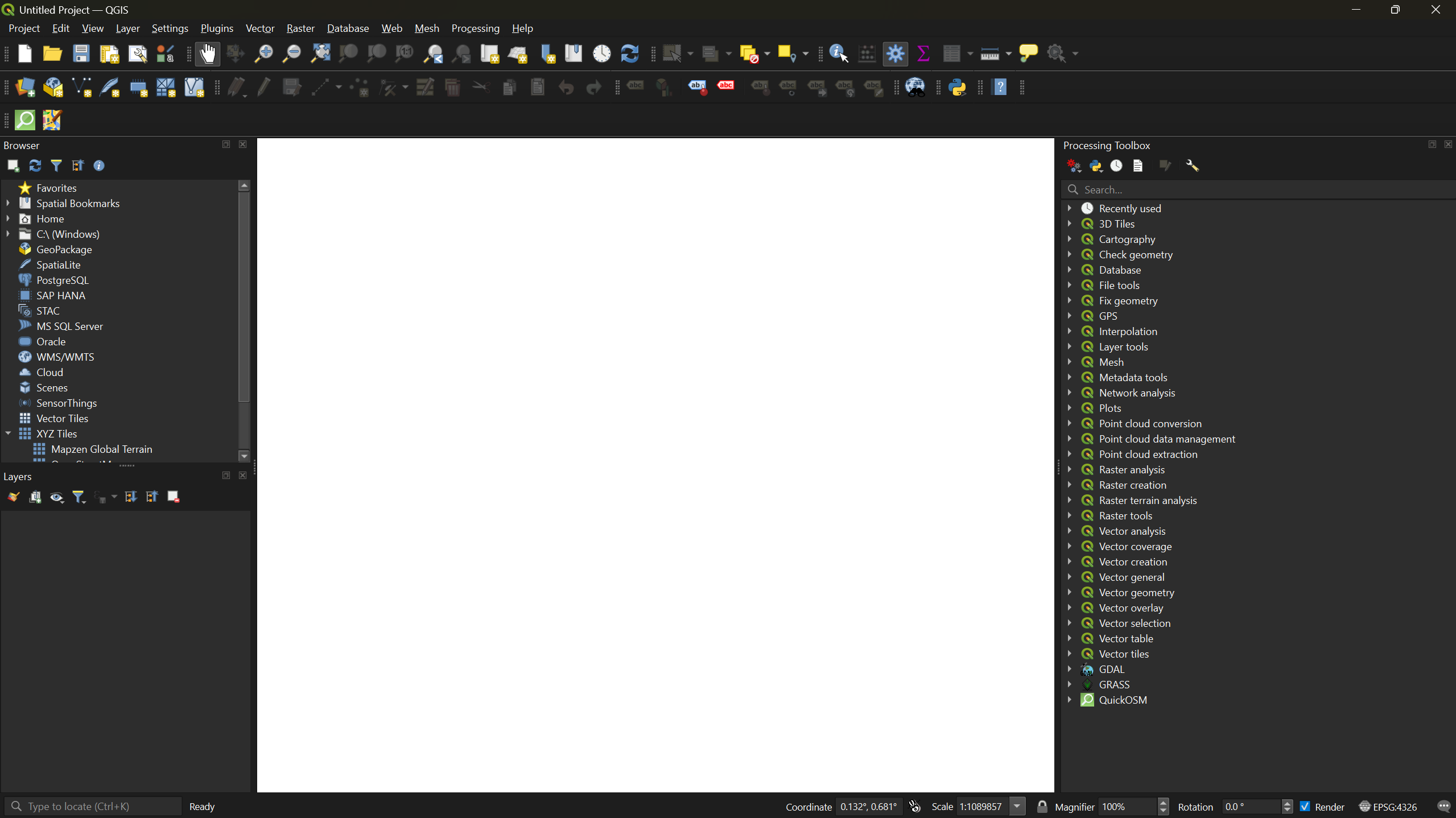
From the menu bar, click Layer → Add Layer → Add Raster Layer. This opens the Data Source Manager.
Click the three-dot button next to Raster dataset(s), navigate to your DEM
.tiffile, and click Open, then Add.
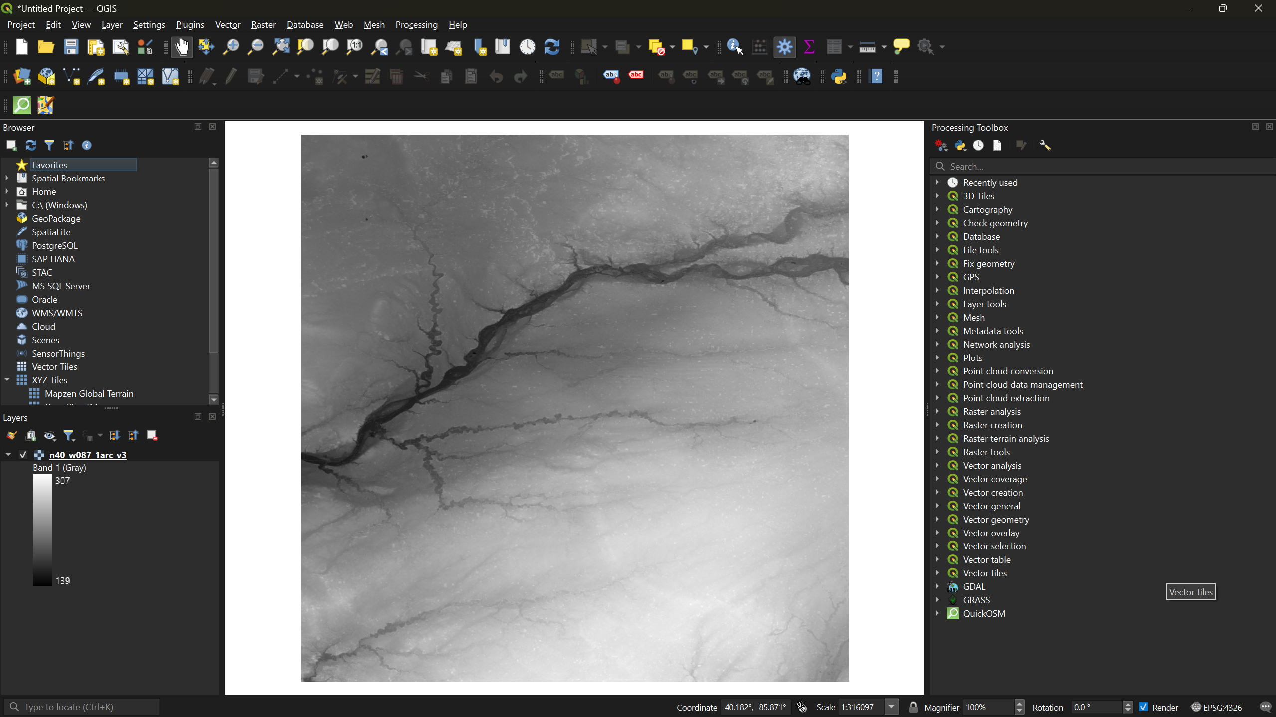
The DEM will appear in grayscale on the map canvas. Darker pixels represent lower elevations and lighter pixels represent higher elevations.
Reprojecting the DEM
The raw DEM uses a geographic coordinate system with units in degrees. For meaningful terrain analysis we need a projected coordinate system that uses meters.
Right-click your DEM layer in the Layers panel and select Properties. Under the Information tab, scroll to Coordinate Reference System (CRS) to confirm the current CRS uses geographic units. Close the dialog.
-
From the menu bar, select Raster → Projections → Warp (Reproject).
- Click the icon next to Target CRS
- Select Predefined CRS from the dropdown
- Search for
26916and select NAD83 / UTM zone 16N - Click Run
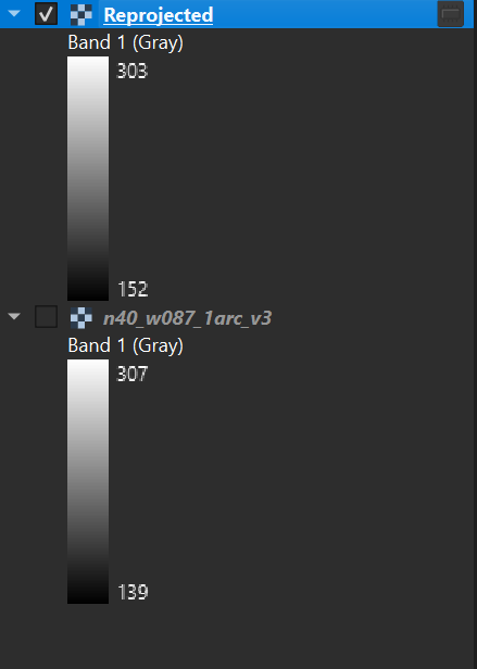
A new layer called Reprojected will appear in the Layers panel.
- Right-click the original DEM layer and select Remove
Layer. Then right-click the reprojected layer, select
Rename Layer, and rename it to
DEM_Analysis.
Why UTM Zone 16N?
This workshop uses study areas in Indiana, which falls within UTM zone 16N. If your area of interest is elsewhere, choose the appropriate UTM zone for your location. Check out this website to find out the correct projection for your region!
Terrain Analysis
With a projected DEM we can now generate three derived layers: slope, aspect, and hillshade. All three are found under Raster → Analysis in the menu bar.
Slope
- Select Raster → Analysis → Slope. Ensure the input
layer is
DEM_Analysisand click Run.
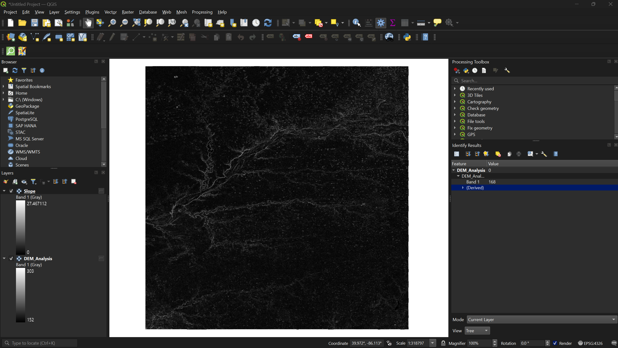
Slope measures how steep the terrain is at each pixel — the rate of elevation change over horizontal distance. Values range from 0° (flat) to 90° (vertical cliff). Slope is commonly used to assess hiking trail difficulty, landslide risk, and water runoff potential.
Aspect
- Select Raster → Analysis → Aspect. Ensure the input
layer is
DEM_Analysisand click Run.
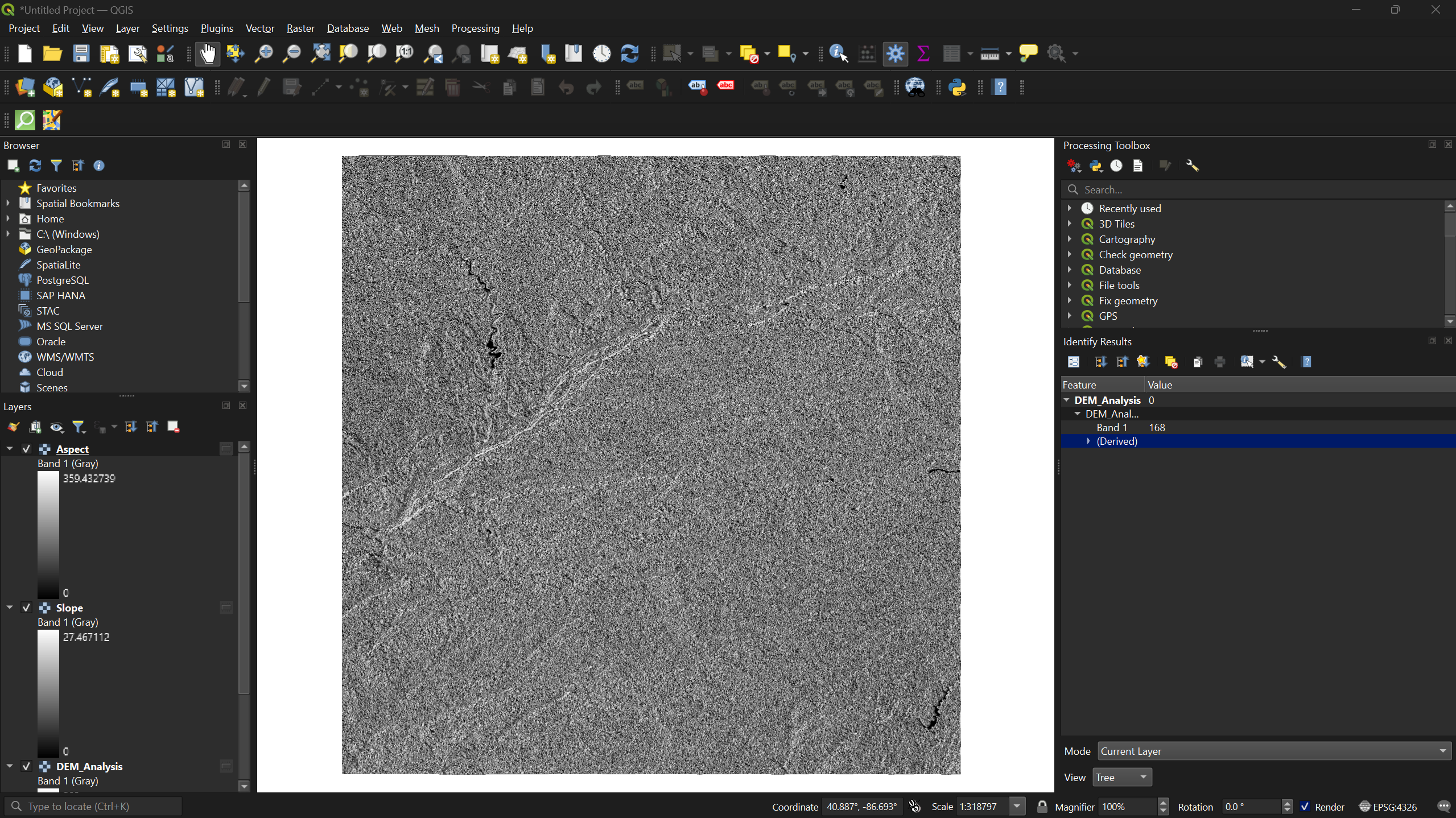
Aspect indicates which compass direction each slope faces. Values run from 0° to 360°, where 0°/360° is north, 90° is east, 180° is south, and 270° is west. Aspect is useful for analyzing sun exposure, vegetation patterns, and snowmelt behavior.
Hillshade
- Select Raster → Analysis → Hillshade. Ensure the
input layer is
DEM_Analysisand click Run.
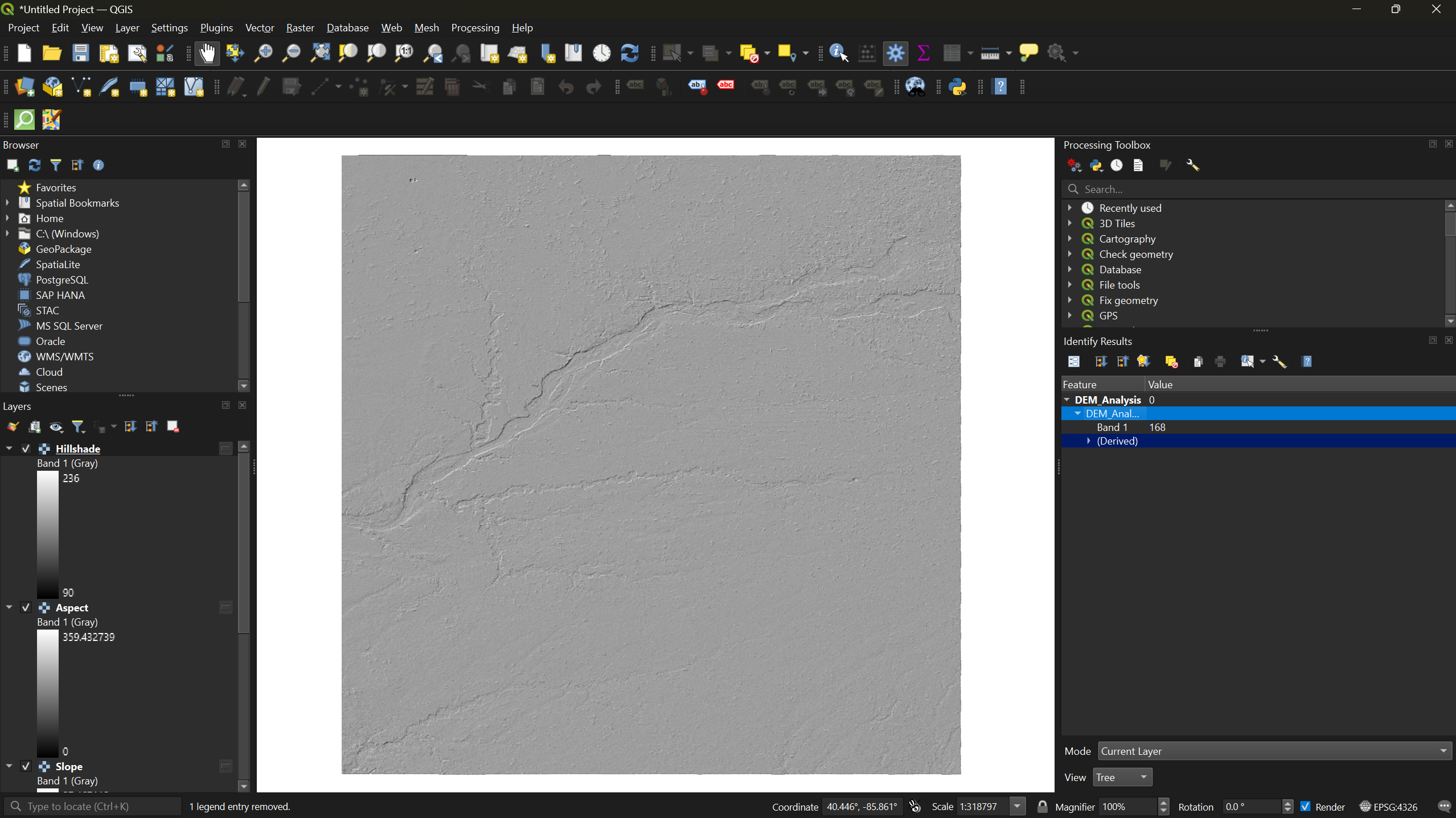
Hillshade simulates how sunlight would illuminate the terrain from a given position. Brighter pixels receive more direct light; darker pixels are in shadow. Hillshade is primarily a visual aid — it makes topography easier to interpret at a glance but does not contain analytical data of its own.
Exercise 1: Compare Terrain Layers
Toggle each of the three layers (slope, aspect, hillshade) on and off in the Layers panel. For your study area, identify a feature that is most visible in one layer but hard to see in another. What does each layer emphasize?
Visualizing Elevation Classes
The grayscale DEM is hard to read. Applying a color ramp makes elevation patterns much easier to interpret.
In the Layers panel, uncheck every layer except
DEM_Analysisso only the original DEM is visible.Right-click
DEM_Analysis, select Properties, and navigate to the Symbology tab.-
Change the Render type from Singleband gray to Singleband pseudocolor. Then:
- Set the Color ramp to Spectral
- Set the Mode to Equal Interval
- Click Classify, then Apply, then OK
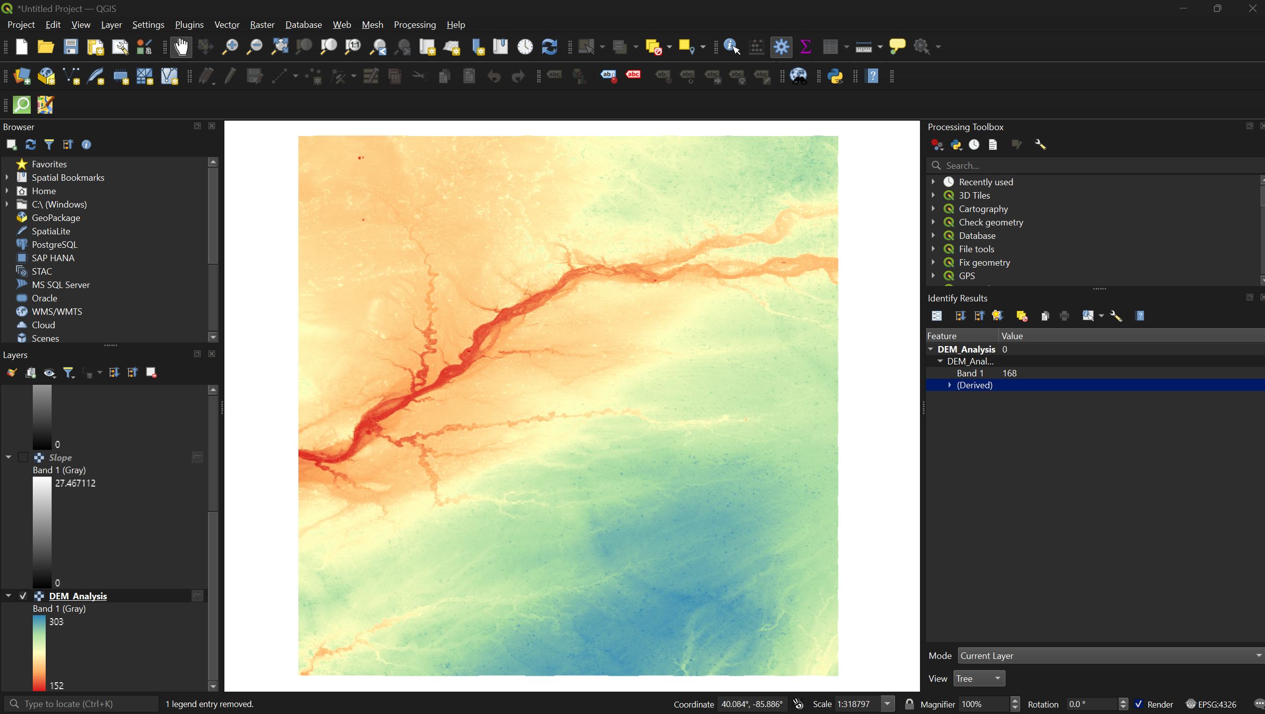
Equal interval divides the full elevation range into classes of equal size. You can adjust the number of classes to the right of the mode selector — try different values and classification modes (e.g., quantile) to see how the visualization changes.
Exercise 2: Experiment with Symbology
- Reopen the Symbology tab for
DEM_Analysis - Try changing the classification mode from Equal Interval to Quantile — how does the map change?
- Try a different color ramp (e.g., Viridis or Magma)
- Increase or decrease the number of classes
Which combination do you think communicates the terrain most effectively?
- DEMs should be reprojected to a metric coordinate system (such as UTM) before performing terrain analysis.
- Slope, aspect, and hillshade are derived layers that each reveal different characteristics of the terrain.
- Pseudocolor symbology with classified elevation ranges makes DEM data far more readable than the default grayscale.