
Raster Processing in Python
Last updated on 2026-10-20 | Edit this page
Overview
Questions
- How do I combine and reclassify rasters cell by cell?
- How do I summarize a raster inside polygons such as census tracts?
- How can land cover improve population estimates?
Objectives
- Explain when rasters line up, and choose a resampling method for measurements and categories
- Make Boolean rasters with comparisons, reclassify categories with a lookup table, and combine rasters
- Compute zonal statistics for measurements and class shares for categories
- Compare dasymetric estimation with areal weighting
What raster analysis adds
Vector operations ask where features are. Raster analysis asks what is everywhere: the elevation of every 30 m cell, the land cover of every cell, the temperature or vegetation index across a whole city. Two families of operations cover most everyday work:
- Map algebra combines rasters cell by cell to make new rasters: arithmetic (elevation in feet), comparisons (land below 170 m), logic (low and developed) and reclassification (16 land cover codes into 5 groups).
- Zonal statistics summarize the cells inside polygons and write the result into the polygons’ table: the mean elevation of each tract, or how many of its cells are developed. This is how raster data meets Census data.
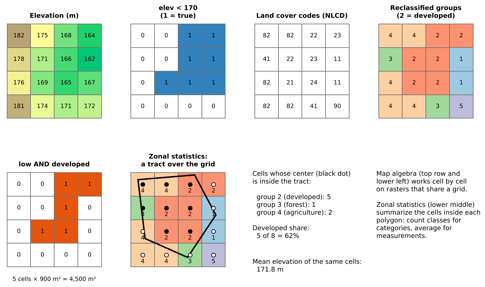
This episode asks two questions about Tippecanoe County, Indiana:
- How much developed land lies close to river level, below 170 m? (A rough stand-in for land near the Wabash River. It is not a flood map; FEMA flood zones are the real source for that.)
- How developed is each census tract, and how does that relate to where people live?
Rasters must line up
Map algebra compares cell (row 10, column 20) of one raster with cell (row 10, column 20) of another, so both must describe the same piece of ground: the same CRS, the same cell size and the same extent and alignment. The two rasters in this episode were prepared that way (EPSG:26916, 30 m cells, one grid). Real data rarely is, and aligning it means resampling:
| Data | Resampling method | Why |
|---|---|---|
| Measurements (elevation, temperature) | Bilinear or cubic | Averages neighboring values smoothly |
| Categories (land cover, zoning codes) | Nearest neighbor | Averaging codes would invent classes that do not exist (the mean of 21 and 41 is 31, “barren”) |
Resample as few times as possible, and to the coarser of the two resolutions: resampling to finer cells adds no information.
Map algebra in four kinds
Map algebra operations are often grouped by how many cells feed each output cell:
| Kind | Each output cell uses | Example |
|---|---|---|
| Local | The same cell in one or more rasters |
elev < 170, low AND developed,
reclassification |
| Focal | A neighborhood around the cell | Slope, hillshade, a 3 by 3 average (Workshop Session 2A’s DEM analysis) |
| Zonal | All cells in the same zone | Mean elevation per tract |
| Global | The whole raster | Distance to the nearest river cell |
This episode uses local and zonal operations.
Reclassification
Reclassification maps old values to new ones with a table. For categories it groups detailed classes; for measurements it cuts a continuous range into classes (0 to 2% slope = flat, and so on). Two checks prevent silent errors:
- Every value must be covered. A code missing from the table becomes no data (or keeps its old value, depending on the software), and the totals no longer add up.
- Range boundaries matter. “11 to 12” can mean 11 < value ≤ 12 or 11 ≤ value ≤ 12. For whole-number codes include both ends.
The groups used here:
| Group | NLCD codes | Meaning |
|---|---|---|
| 1 Water | 11, 12 | Open water, ice |
| 2 Developed | 21 to 24 | Open space (lawns, parks) to high intensity (downtown, industry) |
| 3 Forest and natural | 31, 41 to 43, 52, 71 | Barren, forest, shrub, grassland |
| 4 Agriculture | 81, 82 | Pasture and crops |
| 5 Wetlands | 90, 95 | Woody and herbaceous wetlands |
Zonal statistics
Zonal statistics need the polygons and the raster in the same CRS (software may reproject on the fly, but doing it yourself avoids surprises). Choose the statistic by the kind of raster:
- Measurements: mean, minimum, maximum, range, standard deviation.
- Categories: count of each class (a zonal histogram), then shares. Never average land cover codes.
Most tools count a cell if its center falls inside the polygon. For large polygons this hardly matters; for polygons only a few cells wide (a small park, a narrow tract) the result can be off by a lot. Use finer data, an “all touched” option, or report the limitation.
From land cover to people: dasymetric estimation
In the Geoprocessing episode, areal weighting spread each tract’s population evenly over its area. Land cover lets us do better: people live on developed land, so a piece of a tract that is all farmland should get few of its residents. Dasymetric estimation splits each tract’s population in proportion to its developed cells rather than its area. For Lafayette and West Lafayette it raises the estimated city population from about 114,000 to about 122,000 (edge tracts are partly farmland outside the city limits), while the share within 1 mile of a supermarket barely moves (68% either way). Comparing two methods like this shows how much a conclusion depends on an assumption.
Pitfalls
- No data. Cells outside the county hold a no-data value (here 0 for land cover, -9999 for elevation). Count or average them by mistake and every statistic shifts.
- Units. Areas come from cell counts × cell area, which is only meaningful in a CRS measured in meters.
- Resolution versus polygon size. A 30 m raster says little about a 50 m wide parcel.
- Classification error. Land cover maps come from satellite classification and contain errors, especially between similar classes (pasture and grassland, low and medium intensity developed). Check suspicious results against imagery.
- Date. NLCD 2021 and ACS 2020-2024 are close in time; mixing data decades apart is not.
The same analysis in QGIS
The Raster Processing in QGIS episode does the same steps with the Raster Calculator, Reclassify by table, Zonal statistics and Zonal histogram, on the same data, and reaches the same numbers.
The workflow in code
PYTHON
import rasterio, numpy as np
from rasterstats import zonal_stats

elev = rasterio.open(dem_url).read(1, masked=True)
cover = rasterio.open(lc_url).read(1, masked=True)

low = elev < 170                                    # local: comparison
lookup = np.zeros(256, dtype="uint8")
lookup[[21, 22, 23, 24]] = 2                        # reclassify with a lookup array (other groups likewise)
developed = lookup[cover.filled(0)] == 2
low_developed = low & developed                     # local: combine
print(low_developed.sum() * 900 / 1e6, "km2")      # cells x cell area

stats = zonal_stats(tracts, dem_url, stats=["mean"])                # zonal: measurement
counts = zonal_stats(tracts, lc_url, categorical=True, nodata=0)    # zonal: class counts
Challenge 1: Which resampling?
You need to combine a 10 m land cover raster with a 30 m elevation raster. Which raster would you resample, to what cell size, and with which method?
Resample the land cover to 30 m (the coarser resolution), with nearest neighbor, because it holds categories: bilinear would average codes into classes that do not exist. Resampling the elevation to 10 m would create a finer grid without adding information.
Challenge 2: Mean or count?
For each tract you want (a) its average elevation, (b) its share of forest, and (c) its most common land cover class. Which zonal statistic gives each?
-
Mean of the elevation raster. (b) Counts
per class of the land cover raster
(
categorical=True, or a zonal histogram), then forest cells divided by all cells. (c) The majority (mode) of the land cover raster, whichrasterstatsoffers as"majority". Never the mean of land cover codes.
Challenge 3: When would dasymetric fail?
Dasymetric estimation moves people onto developed land. Name a kind of tract where that assumption works badly, and say why.
Examples: a tract dominated by a shopping center, airport or industrial park (developed but with few residents), so people are placed in parking lots; a university campus, where much developed land is classrooms and labs while residents live in a few dormitories; a rural tract where homes are scattered on farmland classed as agriculture. Weighting developed intensity classes differently, or using building footprints or address points, reduces these errors.
- Map algebra works cell by cell on rasters that share CRS, cell size and extent; resample categories with nearest neighbor
- Comparisons make Boolean rasters, lookup tables reclassify codes,
and
&combines conditions - Zonal statistics summarize cells inside polygons: means for measurements, class counts for categories
- Cell counts times cell area give areas, in a CRS measured in meters
- Dasymetric estimation uses land cover to place people; compare it with areal weighting
Notebooks
| Notebook | What you will do |
|---|---|
| 3a. Map Algebra and Reclassification | Find land below 170 m, group NLCD land cover, and measure developed land near river level; save a GeoTIFF |
| 3b. Zonal Statistics | Mean elevation and percent developed for every tract, relate land cover to density, and compare dasymetric and areal weighting estimates |