NDVI Analysis

Estimated time: 85 minutes

Overview

Questions

• What is NDVI and why is it useful?
• How do we read Landsat bands and compute NDVI in Python?
• How can we classify NDVI into land cover groups?
• What affects NDVI values, and how should they be interpreted?

Objectives

• Explain why vegetation is bright in near infrared and dark in red
• Read raster bands with rasterio and convert them to surface reflectance
• Compute, map and save NDVI as a GeoTIFF
• Classify NDVI with thresholds and summarize area by class
• Describe spectral signatures, image processing levels and resolution
• Recognize the limits of NDVI (season, clouds, saturation, mixed pixels) when comparing places and dates

Why NDVI?

---

Healthy leaves absorb red light for photosynthesis and strongly reflect near infrared (NIR) light. The Normalized Difference Vegetation Index (NDVI) uses that contrast to measure greenness from satellite images. It is easy to compute, works with most sensors (Landsat, Sentinel-2, MODIS), and is used for crop monitoring, drought, urban green space and land cover change.

NDVI	Typical surface
below 0	Water, snow, clouds
0 to 0.2	Bare soil, buildings, roads
0.2 to 0.4	Sparse vegetation, grass, early crops
above 0.4	Dense, healthy vegetation

The notebooks use one Landsat scene over Indiana (Collection 2 Level-2 surface reflectance). For Landsat 8 and 9, Band 4 is red and Band 5 is NIR.

How satellites see vegetation

---

A satellite sensor measures how much sunlight each patch of ground reflects in several bands, narrow ranges of wavelength. The share of light reflected is the reflectance, from 0 (all absorbed) to 1 (all reflected). Each kind of surface has a typical pattern of reflectance across wavelengths, its spectral signature.

Spectral signatures of vegetation, soil and water.

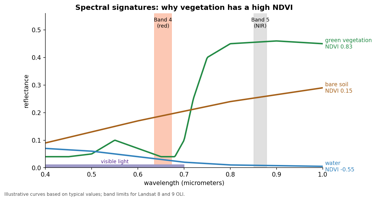
• Healthy vegetation absorbs most red and blue light, because chlorophyll uses it for photosynthesis, and reflects a little more green, which is why leaves look green. In the near infrared, just beyond what our eyes can see, the internal structure of leaves scatters light strongly, so reflectance jumps to 0.3 to 0.5.
• Bare soil and pavement reflect a moderate amount, rising gently with wavelength, so red and NIR are similar.
• Water absorbs nearly all NIR light, so it is dark in that band.

NDVI uses the steep rise between red and NIR (the red edge) that only vegetation shows.

Why a normalized difference?

---

The plain difference, NIR minus red, already separates vegetation from other surfaces, but it also changes with the brightness of the scene: the sun angle, slopes facing toward or away from the sun, and thin haze. Dividing by NIR plus red cancels much of that brightness effect and keeps every value between -1 and +1, so NDVI from different places and dates is easier to compare.

From pixels to reflectance

---

Landsat images are distributed at different processing levels:

Product	What the values are	Use
Level-1	Digital numbers (DN): calibrated sensor counts, still affected by the atmosphere	Needs conversion before indices are compared
Level-2 surface reflectance	Reflectance corrected for the atmosphere, stored as integers	Ready for NDVI after applying the scale and offset

Collection 2 Level-2 values are stored as integers to save space; multiplying by 0.0000275 and adding -0.2 turns them back into reflectance. The value 0 marks pixels outside the scene. Level-2 products also include a QA_PIXEL band that flags clouds, cloud shadows, snow and water. Masking the flagged pixels before analysis stops a cloud from being counted as bare ground.

Resolution describes how much detail an image holds:

	Landsat 8 and 9	Sentinel-2
Pixel size (red and NIR)	30 m	10 m
Red and NIR bands	Bands 4 and 5	Bands 4 and 8
Revisit	16 days per satellite, 8 days with both	About 5 days with both satellites
Archive	Landsat images since 1972 (this sensor design since 2013)	Since 2015

Instructor Note

Pause after the formula and make sure learners know which band is which. Each band is about 90 MB and is read from GitHub into memory, so the reading cell takes a few seconds.

1. Read the bands and convert to reflectance

---

PYTHON

import numpy as np
import matplotlib.pyplot as plt
import rasterio

# rasterio reads the bands straight from GitHub into memory; nothing is downloaded
LANDSAT = "https://raw.githubusercontent.com/SpatialTurn/DataAnalysis/main/data/landsat"

with rasterio.open(f"{LANDSAT}/band4.TIF") as src:     # red
    red = src.read(1).astype("float32")
    profile = src.profile
with rasterio.open(f"{LANDSAT}/band5.TIF") as src:     # near infrared
    nir = src.read(1).astype("float32")

red[red == 0] = np.nan          # 0 = outside the scene
nir[nir == 0] = np.nan

# Level-2 values are stored as integers; this converts them to reflectance (0 to 1)
red = np.clip(red * 0.0000275 - 0.2, 0, 1)
nir = np.clip(nir * 0.0000275 - 0.2, 0, 1)

2. Compute and map NDVI

---

PYTHON

ndvi = (nir - red) / (nir + red)

plt.imshow(ndvi, cmap="RdYlGn", vmin=-0.2, vmax=0.8)
plt.colorbar(label="NDVI")
plt.title("NDVI, Landsat scene over Indiana")
plt.show()

3. Save NDVI as a GeoTIFF (optional)

---

PYTHON

profile.update(dtype="float32", count=1, nodata=np.nan)
with rasterio.open("ndvi.tif", "w", **profile) as dst:
    dst.write(ndvi.astype("float32"), 1)

Everything above stays in memory. Save a file only if you want to open the result in QGIS; it keeps the scene’s location, so it lines up exactly.

4. Classify NDVI

---

np.digitize gives each pixel a class number. Three break values make four classes, so we need four colors.

PYTHON

from matplotlib.colors import ListedColormap

classes = np.digitize(ndvi, [0, 0.2, 0.4]).astype("float32")   # 0, 1, 2, 3
classes[np.isnan(ndvi)] = np.nan

colors = ["#2b83ba", "#d7a26b", "#a6d96a", "#1a9641"]   # water, bare, sparse, dense
plt.imshow(classes[::4, ::4], cmap=ListedColormap(colors), vmin=0, vmax=3,
           interpolation="nearest")    # every 4th pixel keeps the plot fast
plt.title("NDVI classes")
plt.show()

Challenge

Challenge 1: Five classes

Classify NDVI into five classes with breaks [0, 0.1, 0.2, 0.3]. How many colors do you need?

Show me the solution

Four breaks make five classes, so you need five colors and vmax=4.

PYTHON

classes = np.digitize(ndvi, [0, 0.1, 0.2, 0.3]).astype("float32")
classes[np.isnan(ndvi)] = np.nan
colors = ["#2b83ba", "#d7a26b", "#fdae61", "#a6d96a", "#1a9641"]
plt.imshow(classes[::4, ::4], cmap=ListedColormap(colors), vmin=0, vmax=4,
           interpolation="nearest")
plt.show()

Challenge

Challenge 2: Mask water

Replace NDVI values below 0 with np.nan and map the result. What is the mean NDVI of land only?

Show me the solution

PYTHON

ndvi_land = np.where(ndvi < 0, np.nan, ndvi)
plt.imshow(ndvi_land[::4, ::4], cmap="YlGn", vmin=0, vmax=0.8)
plt.show()
print(np.nanmean(ndvi_land))

Masked pixels are left blank on the map and ignored by np.nanmean.

Interpreting NDVI carefully

---

• Thresholds depend on place and season. The table at the top is a rule of thumb. A dry grassland in August and a corn field in July can differ widely. Check thresholds against a true color image or a field visit.
• Saturation. In dense forest and crops, NDVI levels off around 0.8 to 0.9 and stops responding to further increases in leaf area.
• Soil background. Where vegetation is sparse, the soil underneath strongly affects NDVI. The Soil Adjusted Vegetation Index (SAVI) and the Enhanced Vegetation Index (EVI) were designed to reduce soil and atmospheric effects.
• Mixed pixels. A 30 m pixel in a city can contain a tree, a roof and a road. Its NDVI is a blend, so small green spaces such as street trees and yards are underestimated.
• Clouds and shadows lower NDVI and can be mistaken for bare ground or water.

Comparing dates: change detection

---

Subtracting NDVI from two dates (for example ndvi_2024 - ndvi_2014) maps where vegetation was gained or lost. Use scenes from the same time of year, because crops and trees change through the seasons (their phenology), and use the same processing level, ideally from the same or a cross-calibrated sensor. Small differences of a few hundredths are within the noise; look for large, coherent changes.

From thresholds to classification

---

Thresholding NDVI (Section 4) is the simplest way to classify land cover. Notebook 4c goes further:

• Unsupervised classification (K-Means) groups pixels with similar values across several bands; you name the groups afterwards.
• Supervised classification (Random Forest) learns from training samples you label, such as polygons of known forest, water and buildings, and then predicts every pixel. It needs good training data and an accuracy assessment: compare the predictions with reference points that were not used for training, and summarize the agreement in a confusion matrix.

Challenge

Challenge 3: NDVI by hand

Compute NDVI for three pixels and say what each one probably is:

1. red = 0.08, NIR = 0.40
2. red = 0.20, NIR = 0.24
3. red = 0.06, NIR = 0.03

Show me the solution

1. (0.40 - 0.08) / (0.40 + 0.08) = 0.32 / 0.48 = 0.67: dense, healthy vegetation
2. (0.24 - 0.20) / (0.24 + 0.20) = 0.04 / 0.44 = 0.09: bare soil, a road or a roof
3. (0.03 - 0.06) / (0.03 + 0.06) = -0.03 / 0.09 = -0.33: water

Callout

NDVI changes with the seasons, clouds and the atmosphere. Compare scenes from the same time of year, and use surface reflectance (Level-2) products rather than raw Level-1 values when possible.

Math

---

\[ NDVI = \frac{NIR - Red}{NIR + Red} \]

NDVI ranges from -1 to +1. Healthy vegetation has high NIR and low red reflectance, which pushes NDVI toward +1. Water reflects more red than NIR, so its NDVI is negative.

Key Points

• NDVI compares NIR and red reflectance; for Landsat 8 and 9 these are bands 5 and 4
• Convert Level-2 values to reflectance (value * 0.0000275 - 0.2) before computing NDVI
• rasterio reads and writes rasters; reuse the input profile when saving
• np.digitize turns NDVI into classes; n breaks give n + 1 classes
• Vegetation’s spectral signature (low red, high NIR) is what NDVI measures; normalizing reduces brightness effects
• Interpret NDVI with care: thresholds vary, dense canopies saturate, pixels mix, and clouds and seasons change the values

Notebooks

---

Level	Notebook	What you will do
Beginner	4a. Computing NDVI from Landsat	Read bands, convert to reflectance, map NDVI and save a GeoTIFF
Intermediate	4b. Classifying NDVI	Group NDVI into classes, map them and measure area per class
Advanced	4c. Image Classification with Machine Learning	True color image, K-Means and Random Forest classification