Cartography in QGIS

Estimated time: 90 minutes

Overview

Questions

• How do I turn a correct map into a finished one that others can read and print?
• How should layers, labels and a basemap be ordered and styled?
• When do small multiples need a shared scale?

Objectives

• Style and order layers by their role: subject, supporting features, context and reference
• Label features legibly and by rule, with halos
• Add a basemap responsibly, a locator inset, a true scale bar and a north arrow
• Use rule-based styling and labeling, and build a print layout with a locator inset
• Export maps for print and screen

From a correct map to a finished map

---

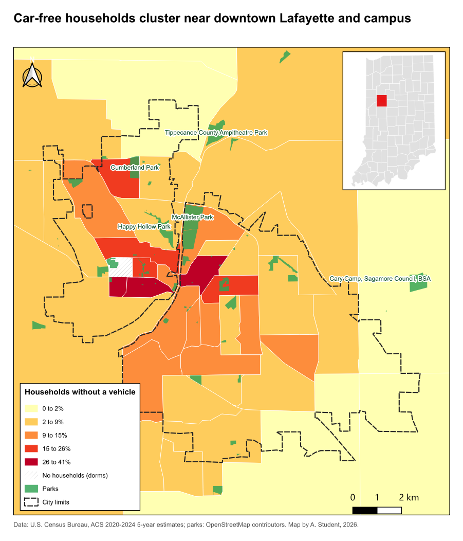
The Fundamentals of Map Design episode covers what a thematic map shows: map elements, normalization, classification and color. This episode is about finishing: turning a correct choropleth into a map that a reader outside your project understands at a glance and that prints cleanly. The running example is the share of households without a car in Lafayette and West Lafayette, Indiana, with parks and city limits on top.

Visual hierarchy, layer by layer

---

Every layer has a role, and its styling should match it:

Role	Example	Styling
Subject	The choropleth of car-free households	Strong color, full opacity
Supporting features	Parks, city limits	Distinct but secondary: one hue, thin or dashed lines, some transparency
Context	Basemap, neighboring areas	Quiet: gray, low contrast
Reference	Labels, scale bar, north arrow, source	Small, legible, never decorative

Order follows from the roles: polygons of the subject at the bottom, supporting outlines and points above them, labels on top, and the basemap underneath everything. A layer on top of a choropleth needs either no fill, transparency, or a strong outline so it does not hide what is underneath.

Labels

---

Labels are reference information. They should be findable, legible and not in the way.

• Label sparingly. Label what the reader needs to orient themselves or to understand the story: the largest parks, the two city names. Labeling all 68 parks makes none of them readable.
• Use a halo (a thin outline in the background color, called a buffer in QGIS). It keeps text readable over any color and is the single most effective labeling technique.
• Use type to signal kind. Common conventions: italics for water and areas (rivers, parks, neighborhoods), upright for places and points, larger or capitalized type for more important names.
• Place labels inside or next to their feature, never across a boundary. For polygons, a point guaranteed to be inside (a “representative point” or “point on surface”) is safer than the centroid, which can fall outside an L-shaped polygon.
• Choose rules, not exceptions. “Label parks over 30 hectares” is reproducible; hand-picking labels is not.

Basemaps

---

A tiled basemap (OpenStreetMap, Esri, CARTO, Stamen) adds streets and place names for free, at a cost: visual noise, a dependence on an online service, and license conditions. Choose a quiet, gray basemap for thematic maps, keep its attribution text, and do not rely on it for print if you need full control or very high resolution. Basemap tiles are in Web Mercator (EPSG:3857); software reprojects them to your map’s CRS, which can blur their labels slightly.

Locator insets, scale bars and north arrows

---

• A locator inset (a small map of the state or country with the study area highlighted) answers “where is this?” for readers who do not know the area. It does not need a scale bar or legend of its own.
• A scale bar is only true on a map in a projected CRS with little distortion over the map (a UTM zone or a state plane for a county). In degrees or Web Mercator at large extents the scale changes across the map, and a single bar misleads.
• A north arrow is only essential when north is not up, but it is cheap and many readers expect one.

Small multiples and shared scales

---

To compare several variables or years, repeat the same map in a grid of small multiples. The eye compares patterns across panels far better than it decodes several variables in one crowded map.

Decide deliberately whether panels share a classification:

• Same variable or same units (one rate in different years, two rates you want to compare): use the same class breaks and colors in every panel, or the same dark color will mean different values.
• Different variables (income in dollars, children in percent): each panel needs its own classes and legend, and the reader compares patterns, not colors.

Export

---

Destination	Format	Notes
Print, a paper, a poster	PDF (vector)	Sharp at any size; set the page or figure size to the printed size
Slides, a website	PNG at 200 to 300 dpi	PNG keeps sharp edges; JPEG blurs lines and text
Further editing (Illustrator, Inkscape)	SVG	Every element stays editable

Check the exported file, not just the screen: font sizes, line widths and legend spacing often look different at print size.

---

Hands-on: a finished map of car-free households

---

These steps were checked in QGIS 4.0. They build on the Foundations episodes Getting Started with QGIS (layers, symbology, print layouts) and Tables, Joins and Selections (virtual fields).

Callout

If QGIS asks you to choose a transformation

When layers in latitude and longitude (EPSG:4326) are drawn in a project in UTM (EPSG:26916), QGIS may open a window titled with “Multiple operations are possible for converting coordinates”. For this county any of the options is accurate to a few meters: keep the first (highlighted) one and click OK. QGIS remembers the choice for the project.

Part 1: Load and order the layers

1. Start a new project and set its CRS to EPSG:26916 (bottom-right corner of the window).

2. Load these with Add Vector Layer, Protocol: HTTP(S), Type: HTTP/HTTPS/FTP:

   Rename to	File
   Tracts	tippecanoe_tracts_acs.geojson
   Parks	tippecanoe_parks.geojson
   City limits	study_area.geojson
   Indiana counties	indiana_counties.geojson
   Tippecanoe County	tippecanoe_county.geojson

   Web addresses to copy:

   • Tracts: https://raw.githubusercontent.com/SpatialTurn/Foundations/main/data/tippecanoe_tracts_acs.geojson
   • Parks: https://raw.githubusercontent.com/SpatialTurn/Foundations/main/data/tippecanoe_parks.geojson
   • City limits: https://raw.githubusercontent.com/SpatialTurn/CaseStudies/main/data/study_area.geojson
   • Indiana counties: https://raw.githubusercontent.com/SpatialTurn/Foundations/main/data/indiana_counties.geojson
   • Tippecanoe County: https://raw.githubusercontent.com/SpatialTurn/Foundations/main/data/tippecanoe_county.geojson

3. Drag them into this order, top to bottom: City limits, Parks, Tracts, Tippecanoe County, Indiana counties. Untick the last two; they are for the locator inset.

4. Style City limits with no fill (Simple Fill, Fill style: No Brush) and a dark dashed outline, and Parks with a green fill, no outline and about 80% opacity (the opacity slider under the symbol).

Check: the dashed city outline and green parks sit on top of the tracts.

Part 2: Rule-based styling with a “no data” class

1. Add a virtual field to Tracts with the Field Calculator: pct_no_vehicle, Decimal (double), "hh_no_vehicle" / "households" * 100.
2. Properties > Symbology: Graduated on pct_no_vehicle, Natural Breaks (Jenks), 5 classes, ramp YlOrRd, white outlines. Click Classify, then Apply.
3. Change Graduated to Rule-based at the top. QGIS converts each class into a rule with a filter such as "pct_no_vehicle" > 2.38 AND "pct_no_vehicle" <= 8.59.
4. Click the green +, give the new rule the filter "pct_no_vehicle" IS NULL, the label “No households (dorms)” and a light gray symbol with a hatch (Fill style: BDiagonal).
5. Double-click each class label and round it (“0 to 2%”, “2 to 9%” and so on). Click OK.

Rule-based symbology converted from Graduated, with a rule for no data.

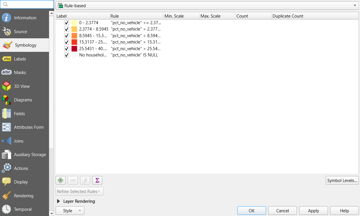
Check: the residence hall tract near campus is drawn in hatched gray instead of disappearing.

Part 3: Labels by rule, with halos

1. Parks > Properties > Labels: choose Rule-based Labeling and click the green +.
2. Filter: $area > 300000 (parks over 30 hectares; $area is in square meters). Value: name.
3. In the rule’s Text tab set the size to about 8 points and a dark green color; in the Buffer tab tick Draw text buffer, size 1 mm, white. That buffer is the halo.
4. Click OK twice.

Rule-based labeling for parks over 30 hectares.

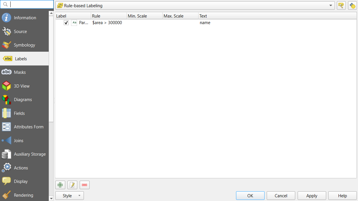
Check: six parks are labeled, each with a white halo. If no labels appear and the numbers in the Preview of $area look far too large, open Project > Properties > General and set Ellipsoid to WGS 84, which is how QGIS measures $area.

Add the two city names as labels in the layout later, or as a small point layer: places are often labeled by hand, in italics.

Part 4: A layout with a locator inset

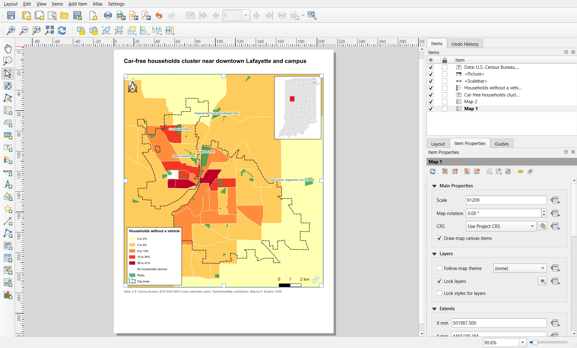
1. Project > New Print Layout, page size Letter (Layout tab, right panel, after right-clicking the page and choosing Page Properties).
2. Main map: Add Item > Add Map, drawn over most of the page. Zoom it to the cities with the Move Item Content tool and the mouse wheel. In Item Properties > Layers, tick Lock layers so the map keeps today’s layers.
3. Locator: in the main QGIS window, tick only Indiana counties and Tippecanoe County (styled gray and red) and zoom to Indiana. Back in the layout, add a second, small map in a corner; tick Lock layers for it too. Then turn the city layers back on in the main window.
4. In the locator’s Item Properties > Overviews, click + and set Map frame to the main map (Map 1). A rectangle shows where the main map is.
5. Add the title (stating the finding), a legend (untick Auto update, remove the county layers, and in the legend panel hide the “Tracts” group heading if you like), a scale bar in kilometers, a north arrow and a source line, as in the Foundations episode.

The print layout with the main map, the locator inset and the map items.

Part 5: Export

1. Layout > Export as PDF for print (vector, sharp at any size).
2. Layout > Export as Image for screens: PNG, with Export resolution 200 to 300 dpi.
3. Open both files and check sizes, fonts and the legend.

The finished map.

Callout

One layout, many maps: atlas

The layout Atlas (Atlas menu in the layout window) repeats a layout once per feature of a coverage layer, for example one page per tract or per county, and exports them all at once. It is the QGIS way to make dozens of consistent maps.

---

Challenge

Challenge 1: What is wrong with this map?

A map of poverty rates by tract uses a satellite basemap at full opacity, red and green classes, labels for every street, a scale bar on a Web Mercator map of the whole United States, and no source line. List the problems and a fix for each.

Show me the solution

• Satellite basemap: too busy for a thematic map; use a quiet gray basemap or none, and keep the attribution.
• Red and green classes: unreadable for many readers with color vision deficiency, and a diverging scheme for a one-directional rate; use a sequential palette (see the Accessibility episode).
• Labels for every street: clutter; label only what orients the reader.
• Scale bar on a national Web Mercator map: the scale varies greatly with latitude; drop it or use an equal-area projection and a note.
• No source line: add the dataset and year.

Challenge

Challenge 2: Two maps, one scale

Make a second layout page (or a second layout) with two maps side by side: car-free households and the poverty rate ("below_poverty" / "poverty_universe" * 100). Should they share classes? Set them up accordingly.

Show me the solution

Both are percentages and the point is to compare them, so share the classes: in both layers use Graduated with Mode: Fixed Interval or manual breaks (edit the values) at 10, 20, 40 and 60%, with the same ramp. Use Lock layers and Lock styles for layers in each map item so each keeps its own layer. One legend is enough. With shared classes it is obvious that poverty rates reach much higher than car-free rates.

Key Points

• Style each layer by its role; the subject is strong, context is quiet
• Convert Graduated to Rule-based to add a “no data” rule; label by rule with a text buffer (halo)
• A second map item with an Overview makes a locator inset; Lock layers keeps each map’s content
• Scale bars need a projected CRS; small multiples share classes only for comparable values
• Export PDF for print and PNG at 200 to 300 dpi for screens, and check the exported file